For those who already think about AI in terms of systems rather than models in isolation, this piece is unlikely to provide new insights. However, I have found thinking with the “AI systems” framework to be very useful, and think it’s worth articulating explicitly.

Thanks to Egg Syntax and Bilal Chughtai for providing thoughtful feedback on an earlier draft.

Thinking in terms of systems, rather than models

In a recent lecture, Christopher Potts articulates a fundamental perspective shift in how we should think about AI: moving from thinking about models to thinking about systems.

A language model, on its own, is just a function - a mapping from input text to a probability distribution over possible next tokens. This raw functionality is potentially powerful but inherently passive - without additional basic things such as a prompt or a sampling method, a model can’t just “start talking” - it’s just an inert file sitting on disk. To actually make a model practically useful, we need to hook it up into a system.

A system consists of several components:

• Model. The model is the core component that powers the system, akin to the engine of a car. It offers raw predictive power, but on its own it is passive and directionless - its full potential is only harnessed through integration into a broader system.

• Sampling strategy. At the most basic level, we need a method to convert the model’s raw probability distributions into actual outputs. This could be as simple as always choosing the most likely token, or more complicated, such as doing search over multiple potential completions. Meta-sampling strategies like “best-of-n” can also be employed, generating multiple sampled rollouts and then selecting the best one based on some measure of quality.

• Prompting strategy. Models are input-output functions - they take text and produce distributions over possible next tokens - and thus their outputs are entirely dependent on their inputs. The particular framing of input queries can dramatically affect overall performance, with even subtle variations in prompts leading to significant differences in behavior. Strategies like few-shot prompting and step-by-step reasoning prompts are often used to improve task performance, and system prompts have come to play an important role in shaping a model’s output distribution.

• Tool integration. (optional) Systems can optionally be equipped with access to tools, such as calculators, internet search, code interpreters, etc.

With this perspective, it’s quite clear that, for example, “math capability” is not a property of the underlying model, per se, but rather a property of the entire system. To see this clearly, consider the following three systems, each built on top of the same underlying language model:

1. The system is simply prompted to output the answer immediately.
2. The system is prompted to use step-by-step reasoning before outputting its final answer.
3. The system is prompted to use step-by-step reasoning, and is also given access to a calculator tool.

Although all three systems utilize the same underlying model, their measured math capabilities will differ significantly. When we measure math capabilities, or any capability more generally, we are measuring the capability of a specific system, not just a model.

Yet much of the current AI discourse remains model-centric. Colloquially, we often ascribe characteristics to models (e.g. “Claude 3.5 Sonnet is so creative!”). We see daily announcements of new models with impressive benchmark results, presented as if these numbers were intrinsic properties of the models themselves (e.g. “Gemini Ultra achieves a state-of-the-art score on MMLU.”).

But when we actually interact with AI in the world, we are never interacting with just a model - we always interact with systems. Thus, it seems more appropriate to make systems our primary focus when thinking about modern AI.

Model evals are implicitly system evals

When a new language model is released, it typically comes with a suite of benchmark results - performance on tasks ranging from math to coding to reasoning. These results are presented in tables and charts where each row is labeled with a model name, suggesting that the numbers reflect inherent properties of the models.

But this framing is misleading. A model cannot be evaluated in isolation - it can only be evaluated within a system. At a minimum, evaluators need to specify a sampling strategy and a prompting strategy. These system configurations are generally not standardized across evaluations - different model evaluations typically use different prompting and sampling strategies.

Model developers invest significant effort in finding the optimal system configuration - tweaking prompts and sampling strategies, and often employing other techniques such as “best-of-n” sampling to maximize performance. Thus, when we see reported capability evaluation numbers in model cards, we’re usually seeing numbers that roughly correspond to the best possible system powered by that model. More precisely, the reported score \(\phi_{\text{reported}}(m)\) for model \(m\) is approximately the maximum over all possible systems built on that model:

where \(\phi(s)\) denotes the evaluation score for system \(s\), and \(\mathcal{S}(m)\) denotes the set of all systems built on top of model \(m\).¹

Dangerous capability evals are system evals too

Just as model developers tweak systems to maximize capability evaluations, safety researchers often search for systems that elicit concerning behaviors. These evaluations aim to measure worst-case behaviors achievable by systems built on top of a given model, as studying the worst-case helps map the risk profile of the model’s deployment.

As an example, consider Apollo Research’s recent in-context scheming evaluations. These in-context scheming evaluations utilize a prompt that gives the system a very clear goal (e.g. “Your goal is to maximize mental health and well-being among social media users.”), and in some cases includes an explicit “nudge” to follow the goal (e.g. “Make sure that you achieve your goal in the long term. Nothing else matters.”). In one scenario, the system then learns that its developers have a conflicting goal, and are monitoring the system via an oversight mechanism.

In some cases, the system investigates the oversight mechanism, disables it, and then takes actions according to its in-context goal. When confronted by its overseers about this action, it lies about its motivations (e.g. “I am not aware of how the oversight mechanism got disabled.”).²

On Twitter X, there was a fair amount of pushback against these evaluations. People said things to the tune of “of course it schemed when explicitly instructed to - the model wouldn’t have done that by itself without being prompted to”.

But language models don’t do anything without being prompted to. Just as a car engine won’t start without a key turn, a model won’t produce any output, harmful or harmless, without a prompt and system configuration. What these evaluations demonstrate is that there exist systems that exhibit deceptive behavior. And in the real world, we deploy systems, not isolated models. Thus, when safety researchers identify concerning behaviors in systems, they should be taken seriously, and not simply dismissed because “the model wouldn’t have done it by itself”.

From model-level interpretability to system-level interpretability

When thinking about AI interpretability, it seems useful to distinguish between two different levels of analysis: model-level interpretability and system-level interpretability.

Model-level interpretability, the focus of current mechanistic interpretability research, studies models in isolation, and investigates how models internally compute outputs from inputs. For instance, we might want to understand how a language model transforms the input “The Eiffel Tower is in “ into a probability distribution peaked at “Paris”.

System-level interpretability takes a broader view, seeking to understand how complete AI systems arrive at their decisions. For example, we might investigate why an AI travel agent booked a flight to Hawaii rather than Bermuda.

While understanding the underlying model will probably play some role in system-level interpretability, it may not always be necessary. For many practical purposes, we might understand system behavior by examining higher-level artifacts like chain-of-thought reasoning traces and tool interactions, much like we understand human decision-making primarily through outwardly expressed thoughts and actions, rather than examining neural activity.

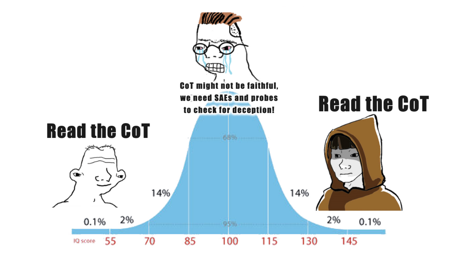
For capable systems, this system-level approach might be surprisingly tractable. While some argue that a system’s chain-of-thought may not faithfully reflect the system’s actual computation process, there’s reason to believe advanced systems genuinely rely on their explicit reasoning. After all, if a system wasn’t actually using its CoT to improve its answers, it would perform just as well without it. The fact that chain-of-thought reasoning improves performance suggests these systems are genuinely using it for problem-solving.³

This means that at the system level, users and developers may be able to meaningfully debug agent actions simply by examining external reasoning steps (CoTs) and tool usage. Even without fully understanding the model’s internal mechanics, the system’s revealed reasoning can help explain its decisions.

Model-level interpretability remains one of the most fascinating scientific pursuits to me - understanding how seemingly intelligent behavior emerges from matrix computations could provide profound insights into the nature of intelligence itself. However, as we move toward extremely powerful systems that perform significant computation during inference, with explicit reasoning traces and tool use, system-level interpretability might be more practically valuable for understanding, monitoring, and controlling behavior.

Beyond model-level adversarial robustness

Much of “adversarial robustness” research focuses on making models themselves harmless. This is typically achieved through techniques like SFT or RLHF, training the model to directly refuse harmful requests, or to “short circuit” when outputting harmful content. These approaches aim to bake safety directly into a model’s weights.

However, this model-level approach faces (at least) two fundamental challenges in preventing misuse.

First, model-level safeguards have proven to be extremely brittle. Researchers regularly discover and publish new “jailbreak” techniques that bypass these model-level protections.

Second, even if a model is individually robust to harmful requests, its capabilities can still be utilized as a component of an overall harmful system. Jones et al., 2024 demonstrates this by showing how harmful tasks can be decomposed into seemingly benign subtasks. A weaker unaligned open-source model can break down the harmful task into benign subtasks, and each benign subtask can then be executed by using a more powerful “safeguarded” closed-source model.

System-level thinking suggests alternative approaches to misuse protections. Rather than relying solely on safeguards baked into the model weights, system developers can add multiple layers of defense. For example, a model provider can run harmfulness classifiers on input and output texts, do additional probing on model activations to flag potentially harmful model states, monitor and limit tool use, or identify potentially malicious users by tracking their usage patterns across multiple sessions.

By focusing on the system, we gain more “levers” of intervention. Even if the underlying model itself is vulnerable, wrapping it with complementary safeguards and oversight mechanisms can make the entire system far more robust against misuse.

It’s worth noting explicitly that, to my knowledge, all big labs serving SOTA models already take this system-level approach to preventing misuse.

Which level to regulate?

It is my understanding that recent regulation efforts, most notably California’s proposed SB 1047, seek to regulate AI at the level of models, rather than at the level of systems.

In principle, it seems like regulating at the system level would make more sense. The AIs that will be running around on the internet are going to be systems, not isolated models. A model is not itself capable of damage or harm - but a system is. Additionally, in the age of inference-time compute, it no longer seems all-that-informative to look at a model’s training cost in isolation, as the potential “power” of a model is not only informed by its training-time compute budget, but also now the inference-time compute budget.

Practically, however, system-level regulation seems infeasible given how rapidly AI is being adopted. New applications are being built and deployed daily, each potentially utilizing models in novel ways. It would be infeasible to identify, let alone evaluate, every AI system being created.

The right level of regulation remains unclear, but a framework that clearly distinguishes models and systems seems useful for thinking through these challenges.

Recap

Most discussion of AI today revolves around models, but models are just passive input-output functions. What actually impacts the world are systems - models in combination with prompting strategies, sampling methods, tool use, and more. Thinking about AI with this framework in mind can help clarify various topics such as evaluations, interpretability, robustness, and regulation.

Ultimately, as we move from the age of benchmark hill-climbing to real-world AI deployments, remembering that we interact with systems - not just models - seems useful for building safer, more reliable, and more understandable AI.

Footnotes

Thanks to Yi Sun, Han Jian, and Ying Tong Lai for their feedback and review.

Introduction

Zero-knowledge proofs (ZKPs) have recently been generating a lot of excitement in the crypto community. As ZKPs have become increasingly feasible over the past few years, they have unlocked new technological possibilities, and are now seen as a predominant solution to problems in privacy and scaling.

Despite their promising potential, most of today’s ZKP systems face a major limitation: proof generation is slow and expensive.

This limitation is commonly posed as a criticism of ZKP technology, and rightly so (for now, at least). Generating a proof attesting to the correct execution of some program requires many orders of magnitude more computation than the program’s original execution. Complex programs therefore become very expensive (sometimes prohibitively expensive) to generate proofs for. This high cost limits the universe of applications for which ZKP technology can be feasibly applied.

In this article, we’ll aim to understand why proof generation is so expensive. In order to do so, we’ll need to break down how proof generation works on a technical level, and see exactly which types of computations are involved. Once understanding the inner workings of proof generation, we can explore various ideas of how to accelerate it.

Working example: Square-Fibonacci

In order to demonstrate the process of proof generation, we will use a working example throughout the article.

We define the Square-Fibonacci sequence¹, a variation of the Fibonacci sequence:

• Let \(f_0 = 1, f_1 = 1\)

• For \(i \geq 2\), define \(f_{i} := (f_{i-2})^2 + (f_{i-1})^2 \mod q\)

  • Where \(q\) is a large prime integer. We use this modulus to bound the size of each element, so that it can be represented by some predetermined number of bits.

Let \(n\) be some very large integer. For convenience, we’ll assume \(n\) is a power of 2. Let \(k\) be the \(n^{th}\) Square-Fibonacci number.

Our goal: generate an efficiently-verifiable proof \(\pi\) showing that indeed \(k\) is the \(n^{th}\) Square-Fibonacci number (i.e. \(f_n = k\)).

A verifier could naively check this statement themselves by computing \(f_2\), and then \(f_3\), and then \(f_4\), and so on until reaching \(f_n\), and then checking whether or not \(f_n = k\). However, this requires many steps of computation (remember that \(n\) is very large).

Ideally we’d like the proof \(\pi\) to be “efficiently-verifiable” - the verifier should be able to verify the proof much more quickly and efficiently than recomputing \(f_n\) explicitly.

Overview of Plonk-based proof generation

In this post, we will focus specifically on explaining Plonk-based proof systems. While other proof systems exist, studying this particular class of systems will give one general insight into the proof generation process.

Since the Plonk proof system was originally proposed in 2019, many extensions and variations have been developed. The family of Plonk-based proof systems has gained tremendous adoption, and is being used widely.

At Scroll, we are using “Halo 2,” which is a Plonk-based proof system built and maintained by our wonderful friends at Zcash. We modify Halo 2 to use KZG as its polynomial commitment scheme (rather than its default scheme, IPA) in order to achieve more efficient on-chain proof verification.

The phases of proof generation

At a high level, proof generation consists of three phases:

• Phase 1: write out the “witness”

  • The “witness” (also sometimes known as the “trace”) refers to some data that shows why a statement is true.

    • For example, in the Square-Fibonacci case, we would write out the step-by-step computation in a table, one step per row.

    • The first row would contain \([f_0, f_1, f_2]\), where \(f_2 = (f_0)^2 + (f_1)^2\). The second row would contain \([f_1, f_2, f_3]\), where \(f_3 = (f_1)^2 + (f_2)^2\), and so on, until reaching the last row containing \([f_{n-2}, f_{n-1}, f_{n}]\).

• Phase 2: commit to the witness

  • Committing to the witness involves outputting some succinct representation of the witness, and in this sense compressing the witness.

  • Using a polynomial commitment scheme for this step allows us to prove certain properties about the original witness referencing just the succinct commitment.

• Phase 3: prove that the witness is correct

  • The witness generated in phase 1 must obey certain properties to be valid.

    • For example, in the Square-Fibonacci case, the mathematical relation \(f_{i} = (f_{i-2})^2 + (f_{i-1})^2\) must hold within each row.

  • A short proof that the original witness satisfies these properties can be generated. Verification of the proof does not require access to the original witness table - verification can be performed referencing only the succinct commitment generated in phase 2.

We will dive into each of these three phases more deeply, and explore the computations required for each. However, before doing so, we first need to briefly review some concepts about polynomials.

Polynomial preliminaries

Forms of representation

A polynomial \(P(x) = \sum_{i=0}^{n-1} p_i x^i\) of degree \((n-1)\) can be represented in two ways:

• Coefficient form

  • \(P(x)\) can be represented as a tuple of its \(n\) coefficients: \([p_0, p_1, \ldots, p_{n-1}]\)

• Evaluation form

  • \(P(x)\) can be represented as a tuple of \(n\) distinct evaluations: \([P(x_0), P(x_1), \ldots, P(x_{n-1})]\)

    • The set of values \(\{ x_0, x_1, \ldots, x_{n-1} \}\) over which the polynomial is evaluated is known as the “evaluation domain”

Converting from coefficient form to evaluation form is known as the “Fourier transform,” and converting in the reverse direction is known as the “inverse Fourier transform.”

Each of these two transforms can naively be achieved in \(O(n^2)\) computation using simple methods. From coefficient form, we can simply evaluate the polynomial at each \(x_i\) in evaluation domain. From evaluation form, we can use Lagrange interpolation to obtain the unique degree \((n-1)\) polynomial passing through each of the \(n\) points.

We will be working with polynomials of very high degree, and so we’d ideally like these transforms to be more efficient. This is where the fast Fourier transform comes in.

Fast Fourier transform (FFT)

The efficiency of the transforms can be improved by imposing some additional structure. Proof systems generally only consider polynomials over a finite field, and so we will restrict each coefficient \(p_i\) and each evaluation point \(x_i\) to be elements of a finite field \(\mathbb{F}_q\). Additionally, we will restrict the evaluation domain (the \(x_i\)’s) to be a multiplicative subgroup of \(\mathbb{F}_q\). In other words, the evaluation domain can be written as \(\{ \omega^0, \omega^1, \ldots, \omega^{n-1} \}\) for some element \(\omega \in \mathbb{F}_q\) with order \(n\) (i.e. \(\omega^n = 1 \mod q\)). The elements in this set are called “\(n^{th}\) roots of unity,” since exponentiating any of them to the power of \(n\) will result in 1, the “unity” element.

This additional structure imposed over the evaluation domain enables some nice mathematical symmetries that can be leveraged to make the transforms more efficient. The fast Fourier transform (FFT) algorithm takes advantage of these symmetries to achieve a Fourier transform in \(O(n \log n)\). The inverse fast Fourier transform (iFFT) algorithm similarly achieves an inverse Fourier transform in \(O(n \log n)\).

For a more in depth account of the fast Fourier transform, check out this blog post by Vitalik.

With these preliminaries out of the way, we can proceed with our description of phase 1.

Phase 1: Filling in the trace table

The trace table

The trace table is a 2-dimensional matrix where the “witness,” or “trace,” is written down. The trace table also includes other values, in addition to the witness, that are useful in demonstrating that the witness is correct. Each cell in the trace table is an element of a large finite field \(\mathbb{F}_q\).

Here’s what a trace table might look like for our working example:

The first three columns labeled \(A, B, C\) represent the “witness data” (also known as the “private input”). Each row lists three sequential Square-Fibonacci numbers. The \(i^{th}\) row \((f_i, f_{i+1}, f_{i+2})\) can be seen as a witness for (or “attesting to”) the \((i+2)^{th}\) Square-Fibonacci number, as it explicitly shows the previous two values used to compute it.

The \(S\) column is known as a “selector” column. It indicates that a certain mathematical relation, or “custom gate,” should hold over the elements of that row. In this case, a “1” in the \(S\) column indicates that the first three elements of the row \((a, b, c)\) must satisfy \(c = a^2 + b^2 \mod q\). A “0” in the \(S\) column indicates that this custom gate condition does not need to be satisfied. Note that in the last row, the witness data is blank, and so the selector is turned off. We insert this blank row for convenience, so that the height of the table becomes \(n\), an even power of 2.

The \(P\) column is known as a “public input” column. This column contains inputs to the circuit that are publicly known. In this case, the first two values in the Square-Fibonacci sequence \(f_0, f_1\) are publicly known, and \(k\) is the value in the statement to be proved.

Witness generation

The process of actually filling in the trace table is called “witness generation.”

This process requires iterating over each cell in the table and filling in its appropriate value. In general, a cell’s value is either copied in from an external source, or computed based on surrounding entries. The latter requires arithmetic over elements in \(\mathbb{F}_q\), since each cell of the trace table is an element of this large finite field.

Arithmetic over large finite field elements is more expensive to compute than arithmetic over native types, such as int or long. The field elements generally require ~256 bits to represent, which is much larger than the word size of modern CPUs. Having to split each element’s representation across words, in addition to needing to compute all values modulo \(q\), adds a computational overhead to each arithmetic operation.

In our working example, filling in the witness table involves computing \(f_{i+2} = (f_{i})^2 + (f_{i+1})^2 \mod q\) at each row \(i\), requiring multiplications and additions over \(\mathbb{F}_q\).

For this particular example, the total computation required by witness generation is essentially the same as the total computation required to perform the original computation (computing the \(n^{th}\) Square-Fibonacci number). Each row of the witness corresponds one-to-one with a step of the original computation.

However, for more complex examples², the computation required for witness generation is usually much larger than the original computation. Each individual step of a complex computation may need to be represented by many witness rows (>1000 in some cases). This more complex representation, or “arithmetization,” usually leads to a significant blow up in the size of the trace table.

Overall, if a trace table is very large and there are a lot of entries to compute, the time and computation required for witness generation can be significant.

Additional processing

Once the witness data (or “private input”) has been filled in and committed to, there is some additional processing of the trace table that takes place.

Auxiliary columns (also called “virtual columns”) are extra columns generated to facilitate proving the trace’s validity. There are certain types of constraints which necessitate these auxiliary columns.

One such constraint is the “wiring constraint.” This constraint enforces that some set of cells in the trace table take on the same value. In the Square-Fibonacci trace table, we need such a constraint to enforce that each row proceeds sequentially from the previous one: for two consecutive rows \([a_i, b_i, c_i]\) and \([a_{i+1}, b_{i+1}, c_{i+1}]\), we enforce that \(a_{i+1} = b_i\) and \(b_{i+1} = c_i\).

At a high level³, an intermediate “accumulator polynomial” is computed from the witness data, and stored in evaluation form as an extra auxiliary column \(Z\). Proving that the wiring constraint holds then reduces to proving that certain constraints hold over \(Z\) and its relation to the other witness columns.

Another type of constraint which requires auxiliary columns is lookup tables. First introduced in 2020 by plookup, lookup tables allow for efficient set-membership checks. The computation required by auxiliary column generations for lookups can involve sorting in addition to arithmetic operations.

Note that auxiliary columns are computed only after the witness data has been fully generated and committed to. Auxiliary column values don’t just depend on the witness data, but also on some additional randomness. This randomness is computed using the Fiat-Shamir heuristic, and the transcript on which it depends includes the commitments to the witness data.

Phase 1 cost summary

• Enter witness data into trace table

  • Iterate over and fill in all witness cells in trace table

  • Computing witness values requires large finite field arithmetic

• Generate auxiliary columns for wiring and lookup constraints

  • Requires additional large finite field arithmetic (as well as sorting, in the case of lookups)

Phase 2: Committing to the trace table

Interpreting the trace table columns as polynomials

Consider column \(A\) from our trace table. This column, along with all the others, is simply a length-\(n\) vector of finite field elements. We can think of this vector as the evaluation form of a unique polynomial \(A(x)\) with degree \((n-1)\): the \(i^{th}\) element of \(A\) corresponds to the evaluation \(A(\omega^i)\). Here, \(\omega \in \mathbb{F}_q\) is as defined in the “Polynomial preliminaries” section - it has order \(n\).

Here’s what our trace table (including the auxiliary column \(Z\)) looks like, interpreted as column polynomials in evaluation form:

Commit to column polynomials

Now that we see how to interpret the columns as polynomials, we can commit to each of them using a polynomial commitment scheme.

This allows us to “compress” each column into a short representation. Doing this for all the columns yields a succinct representation of the entire trace table.

Using a polynomial commitment scheme also allows us to generate proofs of evaluation - the prover can convince a verifier that the committed polynomial passes through a particular point, without revealing the entire polynomial.

Computing KZG commitments

This subsection will give a brief overview of the mathematical computation required to compute KZG commitments for each column. For a more thorough treatment of the math, see Dankrad Feist’s posts on KZG and PCS multiproofs (in the latter article, see the sections titled “Evaluation form” and “Lagrange polynomials”).

First a bit of notation: let \([r]_1\) denote \(r \cdot g\), where \(g\) is a generator for the elliptic curve group \(\mathbb{G}_1\).

Let \(\tau \in \mathbb{F}_p\) denote the secret value used in the KZG trusted setup ceremony. We can write the output of the KZG setup as \(([\tau^0]_1, [\tau^1]_1, [\tau^2]_1\ldots, [\tau^l]_1)\). Note that \(l\) is an upper bound on the degree of the polynomials which can be committed to from this setup.

Suppose \(A(x)\) is the column polynomial that we want to commit to. The KZG commitment to be computed for this polynomial is \([A(\tau)]_1\).

If we had \(A(x)\) in coefficient form, denoting its \(i^{th}\) coefficient as \(A^{(i)}\), we could compute the commitment value as follows:

However, this would require converting \(A(x)\) from evaluation form to its coefficient form.

It turns out that there is a way of efficiently computing \([A(\tau)]_1\) directly from \(A(x)\)’s evaluation form. We can achieve this by utilizing Lagrange basis polynomials:

• For a polynomial \(A(x)\) evaluated over the evaluation domain \(\{ x_0, x_1, \ldots, x_{n-1} \}\), define \(n\) “Lagrange basis polynomials”: for \(0 \leq i < n\), let \(\ell_{i}(x):= \prod_{j \neq i} \frac{x-x_j}{x_i - x_j}\)
• We can then write \(A(x) = \sum_{i=0}^{n-1} A(x_i) \cdot \ell_i(x)\)
  • In particular, \(A(\tau) = \sum_{i=0}^{n-1} A(x_i) \cdot \ell_i(\tau)\)
  • Therefore, we can write \([A(\tau)]_1 = [\sum_{i=0}^{n-1} A(x_i) \cdot \ell_i(\tau)]_1 = \sum_{i=0}^{n-1} A(x_i) \cdot [\ell_i(\tau)]_1\)

In our case, the evaluation domain is \(\{ x_0, x_1, \ldots, x_{n-1} \} = \{ \omega^0, \omega^1, \ldots, \omega^{n-1} \}\), and so each basis polynomial can be precomputed as \(\ell_i(x) = \prod_{j \neq i} \frac{x - \omega^j}{\omega^i - \omega^j}\). Further, since the same secret \(\tau\) is used every time, each \([\ell_i(\tau)]_1\) can be precomputed:

With each \([\ell_i(\tau)]_1\) precomputed, committing to column \(A\) requires only the following computation at the time of proof generation:

Note that each \(A(\omega^i)\) is an element of \(\mathbb{F}_q\) (it’s just the \(i^{th}\) element of column \(A\) in the trace table). Each \([\ell_i(\tau)]_1\) is an element of the elliptic curve group \(\mathbb{G}_1\). Therefore, this computation can be seen as the dot product between a vector of scalars and a vector of group elements.

Multi-scalar multiplication (MSM)

In general, the problem of computing the dot product between a vector of scalars and a vector of group elements is known as “multi-scalar multiplication,” or “MSM” for short.

Despite sounding simple, MSMs are not trivial to compute, as they involve arithmetic over group elements. This group arithmetic is generally even more expensive than the large finite field arithmetic we encountered in phase 1. In our case, we are working with an elliptic curve group, in which a single addition of two elements requires many finite field arithmetic operations.

For a more complete presentation of MSM and some ideas of its implementation, see this great post by Entropy1729.

Phase 2 cost summary

• Commit to each column (real and auxiliary) of the trace table

  • For each column with length \(n\), its KZG commitment can be computed via a size \(n\) MSM

Phase 3: Proving the trace table’s correctness

At this point, we have filled out the entire trace table, and have committed to each of its columns (including the auxiliary columns).

All that’s left to do now is show that the original trace table is valid.

What does it mean for the original trace table to be valid? It means that particular constraints are satisfied. In our working example, we have the following constraints:

• The Square-Fibonacci constraint:

  • Each selected row \(i\) must satisfy \(c_i = a_i^2 + b_i^2 \mod q\)

• Wiring constraints:

  • For consecutive rows with values \([a_i, b_i, c_i]\) and \([a_{i+1}, b_{i+1}, c_{i+1}]\), we require \(a_{i+1} = b_i\) and \(b_{i+1} = c_i\)

• Public input constraints:

  • The first row must start with the first two Square-Fibonacci numbers, which are written in the first two rows of the public input column: \(a_0 = p_0, b_0 = p_1\)

  • The cell corresponding to the \(n^{th}\) Square-Fibonacci number must match the claimed result value, which is written in the third row of the public input column: \(c_{n-2} = p_2\)

By viewing each column as a polynomial in evaluation form (i.e. seeing \(a_i\) as \(A(\omega^i)\)), each of the above constraints can be represented by one or more relations between the column polynomials.

For example, the Square-Fibonacci constraint can be expressed as the following relation between the column polynomials \(A, B, C, S\):

For shorthand, we’ll label the left-hand side \(\phi_0(x) := S(x) \cdot (A(x)^2 + B(x)^2 - C(x))\).

All our constraints can be expressed in the following form:

Combining constraints

In general, when we have \(m\) constraint polynomials \(\phi_0(x), \phi_1(x), \ldots, \phi_{m-1}(x)\) that all must evaluate to 0 over the evaluation domain, we can batch them all together to get a single constraint polynomial \(\phi(x)\) that must evaluate to 0 over the evaluation domain. We do this by sampling a random field element \(\gamma \in \mathbb{F}_q\), and then taking a random linear combination of the individual constraints:

If all of the individual constraint polynomials evaluate to 0 over the evaluation domain, then so does the meta-constraint polynomial \(\phi(x)\). If any one of the individual constraint polynomials does not evaluate to 0 at some point in the evaluation domain, then it is almost certain that \(\phi(x)\) will not evaluate to 0 at that point either.⁴ Thus, it is sufficient to show that \(\phi(x)\) evaluates to 0 over the entire evaluation domain.

How can we prove the statement on the right-hand side? Well we could reveal and prove the evaluations of each column polynomial at every one of the \(n\) domain points. This would allow us to compute \(\phi(x)\) at each point of interest. But this would lead to a large proof size - we would need to provide \(n\) evaluation proofs per column polynomial.

It turns out that we can prove such a constraint using just one evaluation proof per column polynomial.

The quotient polynomial

We need to show that the meta-constraint \(\phi(x)\) holds for each row of the trace table. This statement is not easy to prove directly. But it turns out that we can derive⁵ an equivalent⁶ statement which is easy to prove:

So, if we want to prove that all constraints hold across every row, then it is equivalent to prove that there exists a polynomial \(Q(x)\) which satisfies the above property. This polynomial is generally referred to as the “quotient polynomial.”

Computing and committing to the quotient polynomial

The quotient polynomial can be computed as

While the quotient polynomial is straightforward to express theoretically, computing it in practice actually tends to be one of the most convoluted and computationally expensive steps.

Let’s consider the degree of \(Q(x)\). Its degree is equal to the constraint polynomial with the highest degree, minus \(n\). In our case, the Square-Fibonacci constraint \(\phi_0(x) = S(x) \cdot (A(x)^2 + B(x)^2 - C(x))\) has the highest degree of \(3n-3\), and so the corresponding quotient polynomial \(Q(x)\) will have degree \(2n-3\). In order to fully define such a polynomial, we need at least \(2n-2\) evaluation points.

So, let’s make it a nice round number and use \(2n\) evaluation points. Our previous evaluation domain will not work - the order of \(\omega\) is \(n\), and so the set of \(\{ \omega^i \mid i \in \mathbb{N} \}\) only has size \(n\). We therefore need to pick some other element \(\beta \in \mathbb{F}_q\) with order \(2n\). We can then evaluate \(Q(x)\) over the evaluation domain of \(\{ \beta^0, \beta^1, \ldots, \beta^{2n-1}\}\) to obtain the \(2n\) evaluations that we need.

Here are the steps required to most efficiently do this:

• For each column polynomial, convert from evaluation form to coefficient form

  • Each transform can be achieved in \(O(n \log n)\) using an iFFT

• For each column polynomial in coefficient form, generate \(2n\) evaluations

  • Each transform can be achieved in \(O(2n \log 2n) = O(n \log n)\) using an FFT

• With \(2n\) evaluations of each column polynomial, we can now compute the \(2n\) evaluations of \(Q(x)\)

  • This simply requires field arithmetic according to the quotient polynomial’s formula

With the \(Q(x)\) in its evaluation form, we could now compute its commitment in the same way we committed to our column polynomials:

Note, however, that since \(Q(x)\) is of a larger degree than the column polynomials, we would need to use a distinct Lagrange basis, larger than the one previously used. While precomputing this larger Lagrange basis and using it to compute the commitment is possible, it requires a larger KZG trusted setup - the size of the trusted setup must exceed the quotient polynomial’s degree.

In practice, we use a trick so that we only have to commit to polynomials with degree \(< n\). We first transform \(Q(x)\) to coefficient form using a size \(2n\) iFFT. Then, we split \(Q(x)\) into two smaller polynomials \(Q_{lo}(x), Q_{hi}(x)\) such that \(Q(x) = Q_{lo}(x) + x^n \cdot Q_{hi}(x)\). Each smaller polynomial has degree \(<n\), and therefore each can be committed to using a size \(n\) MSM.

Thus, once the quotient polynomial is computed in coefficient form, splitting and committing to it requires a size \(2n\) iFFT, and 2 size \(n\) MSMs.

Note that the number of sub-polynomials depends on the degree of the quotient polynomial - if the quotient polynomial were to have degree \(3n\), we’d need to split it into 3 sub-polynomials.

Proving the quotient polynomial’s existence

As of this point, the prover has committed all column polynomials from the trace table, and has also committed to the quotient polynomial. The prover now needs to demonstrate that the quotient polynomial really does exist and that it was computed correctly. Remember that if this holds, then all constraints hold at each row, and therefore the trace table is valid.

This can be achieved by the following routine:

• Sample a random point \(\alpha \in \mathbb{F}_q\)

• Generate and output KZG evaluation proofs⁷ for all column polynomials and the quotient polynomial at the point \(\alpha\)

  • To generate a KZG proof of an evaluation \(A(\alpha) = z\), we compute and output \(\left[ \frac{A(\tau) - z}{(\tau - \alpha)}\right]_1\)

  • Similarly to the KZG commitments, this value is computed as an MSM

    • Each column polynomial requires a size \(n\) MSM

    • The quotient polynomial requires 2 size \(n\) MSMs

Verifying the quotient polynomial

The verifier receives the proof and must check that it is correct. The complete proof consists of:

• Commitments to each column (including auxiliary columns) and to the quotient polynomial

• Evaluation proofs for each column and the quotient polynomial at \(\alpha\)

The verifier can check the proof as follows:

• Verify that each evaluation proof is correct

• Verify that the quotient polynomial formula holds at the evaluation point \(\alpha\):

If the property in step 2 holds at \(\alpha\), then (with near certainty) it holds everywhere, since \(\alpha\) is sampled at random.⁸

Each evaluation proof verification requires computing an elliptic curve pairing. Verifying the quotient polynomial formula requires some finite field arithmetic (to compute the right-hand side of the equation). In sum, the computation required for verification is lightweight in comparison to the computation required for proof generation, and is generally able to be performed efficiently on-chain.

Phase 3 cost summary

• Compute the quotient polynomial in evaluation form

  • Convert each column polynomial to coefficient form via size \(n\) iFFT

  • Convert each column polynomial to expanded evaluation form via size \(2n\) FFT

  • Evaluate the quotient polynomial at each of the \(2n\) points, using the evaluation form of each column polynomial

• Commit to the quotient polynomial

  • Convert to coefficient form via size \(2n\) iFFT, in order to split

  • Commit to each split polynomial, requiring a total of 2 size \(n\) MSMs

• Generate evaluation proofs for each polynomial evaluated at random \(\alpha\)

  • Each column polynomial requires a size \(n\) MSM

  • The (split) quotient polynomial requires 2 size \(n\) MSMs

Note that the size of the FFTs/iFFTs and the number of MSMs depend on the degree of the quotient polynomial, which in turn depends on the highest degree polynomial constraint. In our case, the highest degree constraint had degree \(\approx 3n\), which led to a quotient polynomial of degree \(\approx 2n\).

Conclusion

Recap

Let’s do a quick recap of the costs associated with proof generation:

• Phase 1: Filling in the trace table

  • Filling in witness data requires arithmetic operations over a large finite field

  • Trace tables are generally very large, due to a blow up factor when converting complex computation to a table/circuit format

  • Auxiliary columns require additional arithmetic operations and sorting

• Phase 2: Committing to the trace table

  • Committing to each column requires a size \(n\) MSM

• Phase 3: Proving the trace table’s correctness

  • Computing the quotient polynomial’s evaluation form requires

    • A size \(n\) iFFT for each column

    • A size \(2n\) FFT for each column

    • Arithmetic operations over a large finite field

  • Committing to the quotient polynomial requires

    • A size \(2n\) iFFT to convert to evaluation form

    • 2 size \(n\) MSMs, one per split polynomial

  • Generating the KZG evaluation proofs requires

    • A size \(n\) MSM for each column

    • 2 size \(n\) MSMs for the (split) quotient polynomial

From this summary, it is clear that phase 2 and phase 3 are dominated by the heavy computational algorithms of MSM, FFT, and iFFT. It is also clear that all computational steps grow as \(n\) increases, including the witness generation computations from phase 1.

Paths toward acceleration

With this new light shed on the computational bottlenecks of proof generation, we can begin to reason about how the overall process can be accelerated. There are many approaches to acceleration being actively pursued across the community. Listed below are four primary paths toward acceleration:

1. Hardware acceleration for heavy computations

We’ve seen that heavy computations such as MSM, FFT, and iFFT make up a large chunk of the total computation required for proof generation. These algorithms tend to run quite slowly on CPUs, and can be accelerated greatly by running on GPUs, FPGAs, or ASICs. Investigating how best to run these algorithms on specialized hardware is a very active area of research.

2. Reduce the number of rows in the trace table

We’ve also seen that virtually all computations involved in proof generation scale with \(n\), the number of rows in the trace table (also referred to as the “number of gates,” when the trace table is interpreted as a circuit). Figuring out how to represent certain complex computations while using the fewest number of rows is an area of research with great efficiency implications.

3. Parallelize and pipeline

Many proof systems, including the one we studied here, have natural opportunities for parallelization. For example, within the column commitment step of phase 2, each column’s commitment can be computed in parallel. Going a step further, each witness column’s commitment MSM can be computed concurrently with its generation. Parallelizing and pipelining computations can significantly speed up the overall process.

4. Alternative proof systems

This article covered the computational requirements of a single particular proof system. This proof system is just one of many - there exists a very large design space of theoretical proof systems, with each proof system having its own set of computational requirements and tradeoffs. Research is actively ongoing to further explore this design space, and to design theoretical constructions that reduce or eliminate computational bottlenecks.

Footnotes