Attention
Query, key, and value projections
Let \(x \in \mathbb{R}^{n_\text{seq} \times d_\text{model}}\) represent the model’s activations at a particular layer - each \(x_i \in \mathbb{R}^{d_\text{model}}\) is the activation at token position \(i \in [n_{\text{seq}}]\).
For each attention head \(h\), we project each activation \(x_i\) to corresponding query, key, and value vectors:
\[\begin{aligned} q_i^{(h)} &= W_Q^{(h)} x_i, \\ k_i^{(h)} &= W_K^{(h)} x_i, \\ v_i^{(h)} &= W_V^{(h)} x_i, \end{aligned}\]where the linear maps \(W_Q^{(h)}, W_K^{(h)}, W_V^{(h)} \in \mathbb{R}^{d_{\text{head}} \times d_{\text{model}}}\) are learned parameters.
The resulting vectors \(q_i^{(h)}, k_i^{(h)}, v_i^{(h)} \in \mathbb{R}^{d_{\text{head}}}\) live in a much lower-dimensional space than the original activations (i.e. \(d_{\text{head}} \ll d_{\text{model}}\)).
Intuitively, we can think of the projections as follows:
- The query vector \(q_i^{(h)}\) represents what information \(x_i\) looks for.
- The key vector \(k_i^{(h)}\) represents what information \(x_i\) contains.
- The value vector \(v_i^{(h)}\) represents what information \(x_i\) propagates.
Attention mechanism
The main functionality of the attention mechanism is to transfer information between token positions.
In order to determine which information should be transferred to activation \(x_i\) at position \(i\), we check to see which past activations \(\{ x_j \mid j \leq i \}\) contain information that the current activation \(x_i\) is looking for.
We can formulate this using the language of query and key vectors: we check to see which past key vectors \(\{ k_j^{(h)} \mid j \leq i \}\) are similar to the current query vector \(q_i^{(h)}\).
We can compute the similarity between a query vector and key vector by simply taking their dot product:
\[\begin{align*} \text{score}_{i \rightarrow j}^{(h)} = \frac{q_i^{(h)} \cdot k_j^{(h)}}{\sqrt{d_{\text{head}}}}. \end{align*}\]Here, the subscript \(i \rightarrow j\) indicates that position \(i\) looks at position \(j\) - I use this convention throughout.1
Why scale by \(\frac{1}{\sqrt{d_{\text{head}}}}\)?
We scale by \(\frac{1}{\sqrt{d_{\text{head}}}}\) to ensure that the dot products don’t grow with \(d_{\text{head}}\). This scaling is important because larger dot products would cause the softmax function to saturate, resulting in vanishing gradients.
To see how scaling by \(\frac{1}{\sqrt{d_{\text{head}}}}\) prevents the dot products from growing with \(d_{\text{head}}\), let’s assume \(q_i^{(h)}\) and \(k_i^{(h)}\) to be drawn from \(\mathcal{N}(0, I)\). Then \(q_i^{(h)} \cdot k_i^{(h)}\) has a mean of 0 and variance of \(d_{\text{head}}\) - each summand of the dot product is distributed as \(\mathcal{N}(0, 1)\), and there are \(d_{\text{head}}\) such terms (recall that the variance of the sum of independent random variables is the sum of their variances). Scaling the resulting quantity by \(\frac{1}{\sqrt{d_{\text{head}}}}\) results in a variance of \(\left( \frac{1}{\sqrt{d_{\text{head}}}}\right)^2 \cdot d_{\text{head}} = 1\).
For causal attention, we set \(\text{score}_{i \rightarrow j}^{(h)} = -\infty\) for all \(j > i\). This prevents future token positions from transferring information to past token positions.
We then apply a softmax function to the scores to obtain the attention weights:
\[\text{attention}_{i \rightarrow j}^{(h)} = \frac{\exp(\text{score}_{i \rightarrow j}^{(h)})}{\sum_{k=1}^{n_{\text{seq}}} \exp(\text{score}_{i \rightarrow k}^{(h)})}.\]Intuitively, \(\text{attention}_{i \rightarrow j}^{(h)}\) describes how strongly information from token position \(j\) should be transferred to token position \(i\). We operationalize this by weighting each value vector \(v_{j}^{(h)}\) by \(\text{attention}_{i \rightarrow j}^{(h)}\):
\[\begin{align*} \text{weighted\_value}_i^{(h)} = \sum_{j=1}^{n_{\text{seq}}} \text{attention}_{i \rightarrow j}^{(h)} v_j^{(h)}. \end{align*}\]Finally, we map this vector \(\text{weighted\_value}_i^{(h)} \in \mathbb{R}^{d_{\text{head}}}\) back to the original dimension \(d_{\text{model}}\):
\[\begin{align*} \text{attention\_out}_i^{(h)} = W_O^{(h)} \text{weighted\_value}_i^{(h)} + b_O^{(h)}, \end{align*}\]where \(W_O^{(h)} \in \mathbb{R}^{d_{\text{model}} \times d_{\text{head}}}\) and \(b_O^{(h)} \in \mathbb{R}^{d_{\text{model}}}\) are learned parameters.
Multi-head attention
The above description focused on a single head. In practice, we feed the activation \(x_i\) through multiple, say \(n_{\text{heads}}\)-many, attention heads in parallel.
For each head \(h \in [n_{\text{heads}}]\), we compute the attention output \(\text{attention\_out}_i^{(h)}\) as described above. We then sum the outputs across all heads:
\[\text{multi\_head\_attention\_out}_i = \sum_{h \in [n_{\text{heads}}]} \text{attention\_out}_i^{(h)}.\]It is usually the case that \(d_{\text{model}} = d_{\text{head}} \cdot n_{\text{heads}}\). For example, the original transformer in Vaswani et al., 2017 used \(d_{\text{model}} = 512\) with \(n_{\text{heads}} = 8\) and \(d_{\text{head}} = 64\).
KV caching
Once trained, a transformer is generally used to generate sequences of tokens autoregressively - one token at a time.
Consider for a moment how this actually works.
Let’s say we have a prompt \([t_1, \ldots, t_n]\) as input. We want to generate the next token \(t_{n+1}\). We can do this by running the transformer over the whole sequence \([t_1, \ldots, t_n]\), and then sampling \(t_{n+1}\).
Next, we want to generate \(t_{n+2}\). Naively, we could run the transformer over the entire sequence \([t_1, \ldots, t_n, t_{n+1}]\), and then sampling \(t_{n+2}\). But it turns out that this is really wasteful!
There are two key observations to notice:
- In a causal transformer, activations at positions \(1, \ldots, n\) will be exactly the same whether we run the transformer over the sequence \([t_1, \ldots, t_n]\) or \([t_1, \ldots, t_n, t_{n+1}]\). Adding new tokens doesn’t change how previous tokens are processed.
- When running the transformer at position \(n+1\), the only data that is needed from previous token positions are the keys and values.
This leads to an elegant optimization called KV caching. After generating each token, we store the keys and values for all positions processed so far. For each attention head \(h\), we maintain:
\[\begin{aligned} \text{key\_cache}^{(h)} &: [k_1^{(h)}, k_2^{(h)}, \ldots, k_t^{(h)}] \\ \text{value\_cache}^{(h)}&: [v_1^{(h)}, v_2^{(h)}, \ldots, v_t^{(h)}] \end{aligned}\]When running inference at position \(t+1\), we can simply use the cached keys and values to compute the attention output, and also update the cache with new keys and values for position \(t+1\).
This allows us to run the forward pass on just one token position!
However, the cache does incur a memory cost of \(O(2 \cdot n_{\text{seq}} \cdot n_{\text{layers}} \cdot n_{\text{heads}} \cdot d_{\text{head}})\). Doing vanilla forward passes without caching requires \(O(n_{\text{seq}} \cdot d_{\text{model}} + n_{\text{seq}}^2)\) memory - we can store and compute the activations one layer at a time, but need to compute the attention scores for all token pairs.
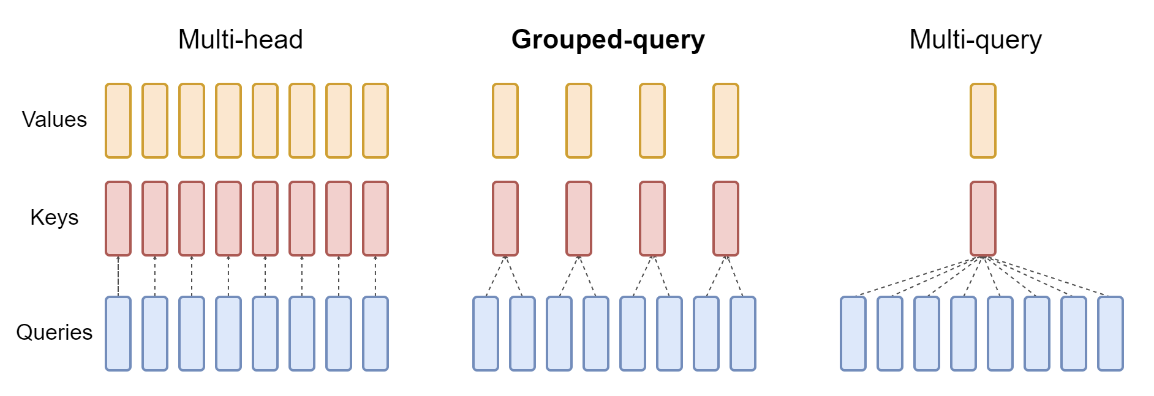
Multi-query attention
Recall that in standard multi-head attention (MHA), each head has its own query, key, and value projections. While this design is very flexible, it can become memory-intensive as the context length grows, since we need to store \(n_{\text{seq}} \cdot n_{\text{layers}} \cdot n_{\text{heads}}\) different sets of keys and values.
Multi-query attention (MQA) changes this by sharing a single set of keys and values across all heads, but still having different queries per head. Concretely:
- We maintain \(n_{\text{heads}}\) different query projections \(W_Q^{(h)}\), so each head still computes its own query vector:
- We now share one key matrix \(W_K\) and one value matrix \(W_V\) for all heads. Hence, the keys and values become the same for each head:
This means each attention head “sees” the same keys and values, but they “look” at them differently via distinct query vectors.
This approach is very memory-efficient, since the memory cost of the KV cache is reduced from \(O(n_{\text{seq}} \cdot n_{\text{layers}} \cdot n_{\text{heads}} \cdot d_{\text{head}})\) to \(O(n_{\text{seq}} \cdot n_{\text{layers}} \cdot d_{\text{head}})\).
However, MQA is not as expressive as standard MHA, since each head must share the same keys and values.
Grouped-query attention
[Source: Figure 2 of Ainslie et al., 2023.]
Grouped-query attention (GQA) is a middle-ground approach between full MHA and MQA. The core idea is to form a smaller number of groups, each group sharing one set of keys and values, but still allowing multiple heads within that group to have distinct queries.
Concretely:
- We partition the \(n_{\text{heads}}\) heads into \(g\) groups.
- Each group \(r \in [g]\) has a shared key projection \(W_K^{(r)}\) and a shared value projection \(W_V^{(r)}\).
- All heads within group \(r\) use the same key and value projections, but each head in that group keeps its own query projection:
GQA is a middle-ground between full MHA and MQA.
Compared to MHA, GQA reduces the memory cost of the KV cache from \(O(n_{\text{seq}} \cdot n_{\text{layers}} \cdot n_{\text{heads}} \cdot d_{\text{head}})\) to \(O(n_{\text{seq}} \cdot n_{\text{layers}} \cdot g \cdot d_{\text{head}})\).
Compared to MQA, GQA is more expressive, because there are multiple K/V sets - one per group - rather than a single shared K/V set across all heads.
Multi-head latent attention
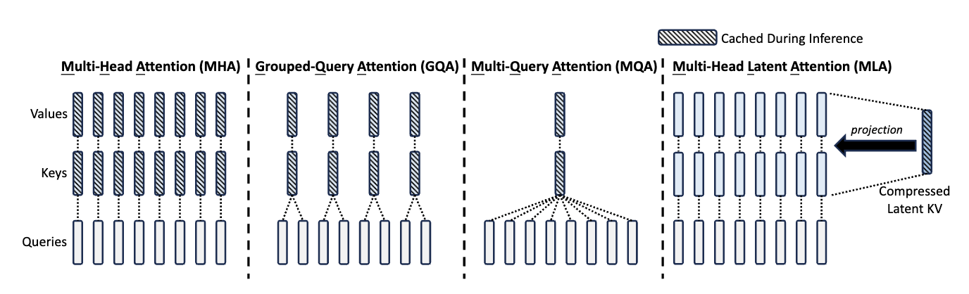
[Source: Figure 3 of DeepSeek-AI, 2024.]
Multi-head latent attention (MLA) is another technique to reduce the memory cost of the KV cache while maintaining model performance.
Given an activation \(x_i\) at position \(i\), we first project it to a compressed latent vector \(c_i^{\text{KV}}\):
\[c_i^{\text{KV}} =W_{\text{DKV}} x_i,\]where \(W_{\text{DKV}} \in \mathbb{R}^{d_c \times d_{\text{model}}}\) is a learned down-projection matrix, projecting from \(d_{\text{model}}\) down to \(d_c\). Note that for this compression to be effective, we choose \(d_c \ll n_{\text{heads}} \cdot d_{\text{head}}\).
This latent vector is then expanded into keys and values for each head:
\[\begin{aligned} k_i^{(h)} &= W_{\text{UK}}^{(h)} c_i^{\text{KV}}, \\ v_i^{(h)} &= W_{\text{UV}}^{(h)} c_i^{\text{KV}}, \end{aligned}\]where \(W_{\text{UK}}^{(h)}, W_{\text{UV}}^{(h)} \in \mathbb{R}^{d_{\text{head}} \times d_c}\) are learned up-projection matrices2, projecting from \(d_c\) to \(d_{\text{head}}\).
For queries, MLA similarly uses a compressed representation:
\[\begin{aligned} c_i^{\text{Q}} &= W_{\text{DQ}} x_i, \\ q_i^{(h)} &= W_{\text{UQ}}^{(h)} c_i^{\text{Q}}, \end{aligned}\]where \(W_{\text{DQ}} \in \mathbb{R}^{d_c' \times d_{\text{model}}}\) is a learned down-projection matrix, and \(W_{\text{UQ}}^{(h)} \in \mathbb{R}^{d_{\text{head}} \times d_c'}\) is a learned up-projection matrix.
During inference, we only need to cache the latent vectors \(c_i^{\text{KV}}\), not the full keys and values. While caching the full keys and values as in MHA requires \(O(n_{\text{seq}} \cdot n_{\text{layers}} \cdot n_{\text{heads}} \cdot d_{\text{head}})\) memory, caching the latent vectors requires only \(O(n_{\text{seq}} \cdot n_{\text{layers}} \cdot d_c)\) memory, where \(d_c \ll n_{\text{heads}} \cdot d_{\text{head}}\).
Another cool property of MLA is that the keys and values don’t need to be computed explicitly. Recall that the attention scores are computed as:
\[\begin{aligned} \text{score}_{i \rightarrow j}^{(h)} &\propto q_i^{(h)} \cdot k_j^{(h)} \\ &= (W_{\text{UQ}}^{(h)} c_i^{\text{Q}})^{\top} (W_{\text{UK}}^{(h)} c_j^{\text{KV}}) \\ &= c_i^{\text{Q}} \underbrace{\left(W_{\text{UQ}}^{(h)}\right)^{\top} W_{\text{UK}}^{(h)}}_{:= W_{\text{UQK}}^{(h)} \in \mathbb{R}^{d_c' \times d_c}} c_j^{\text{KV}}. \end{aligned}\]Thus, we can “roll” \(W_{\text{UK}}^{h}\) into \(W_{\text{UQ}}^{(h)}\), and just compute affinity scores between the compressed query and key vectors.
We can similarly “roll” \(W_{\text{UV}}^{(h)}\) into \(W_{\text{O}}^{(h)}\).
Sparse attention
The techniques above - MQA, GQA, and MLA - all address the memory cost of the KV cache. But there’s another precious resource that we need to consider: compute. For each query at position \(n_{\text{seq}}\), attention considers every preceding key. This means that the computation at position \(n_{\text{seq}}\) is \(O(n_{\text{seq}})\), and so producing \(n_{\text{seq}}\) tokens autoregressively requires \(O(n_{\text{seq}}^2)\) compute.
The key observation is that most post-softmax attention weights end up near zero. I.e., each query attends strongly to only a small subset of preceding tokens - the rest contribute negligibly to the output.
The key idea behind sparse attention is to first identify a small set of candidate key tokens - the ones actually worth attending to - and then to run full attention only over that set. If we always select a fixed \(k\) candidates, then the expensive full-attention step becomes \(O(k)\) per query regardless of context length.
But how do we identify the candidate key tokens? Well, we can scan over all previous tokens and compute some sort of relevance score for each, and then select the top-\(k\) candidates with the highest scores. Note that this still requires scanning all previous tokens to find the candidates, and therefore is still \(O(n_\text{seq})\). But that scan can be much cheaper than full attention. The intuition: answering “is this token worth attending to?” is a simpler question than “how much should I attend to it, and what information does it contain?”, and should therefore be cheaper to compute.
DeepSeek Sparse Attention (DSA) implements this idea, using a “lightning indexer” that scans all previous tokens and assigns a relevance score to each, followed by full attention over only the top-\(k\) candidates.
For the query at position \(i\) and each preceding position \(j\), the indexer computes:
\[I_{i \rightarrow j} = \sum_{h=1}^{H_I} w_{i,h}^I \cdot \text{ReLU}\!\left( q_{i,h}^I \cdot k_j^I \right),\]where \(H_I\) is the number of indexer heads, \(q_{i,h}^I, k_j^I \in \mathbb{R}^{d_I}\) are low-dimensional query and key projections, and \(w_{i,h}^I \in \mathbb{R}\) is a learned scalar weight derived from \(x_i\) that controls how much head \(h\)’s score contributes for this query. The indexer can get away with using fewer heads, lower-dimensional vectors, ReLU (instead of softmax), and running at lower precision. With these simplifications, the indexer can run much more cheaply than normal attention.
The \(k\) positions with the highest scores become the candidate set. Full attention then runs over only those \(k\) entries.
DeepSeek-V3.2 uses a single shared candidate set across all attention heads, rather than letting each head select independently. This is primarily a hardware convenience: per-head selection would create \(n_{\text{heads}}\) different irregular memory access patterns. MLA makes this additionally natural, since the latents are already shared across heads.
Cost analysis
How much compute does attention require per query token? For each preceding position, attention performs a fixed amount of work: computing a query-key dot product (to get the attention score) and weighting the corresponding value (to accumulate the output). Call this per-pair cost \(C\). Since the query at position \(L\) pairs with all \(L\) preceding positions (including itself), the total cost is simply \(C \cdot L\).
For vanilla attention, every pair goes through the full multi-head mechanism, so:
\[\text{FLOPs}_\text{vanilla}(L) = C_\text{attn} \cdot L.\]For DSA, two different operations run at different costs: the indexer scans all \(L\) tokens (at \(C_\text{idx}\) per pair), then full attention runs on only \(k\) of them (at \(C_\text{attn}\) per pair):
\[\text{FLOPs}_\text{DSA}(L) = C_\text{idx} \cdot L + C_\text{attn} \cdot k.\]Let’s estimate \(C_\text{attn}\) and \(C_\text{idx}\) for DeepSeek-V3.2. For each (query, key) pair, full MLA attention does two things per head: a QK dot product over \(d_c = 512\) dimensions (\(2d_c\) FLOPs), and a value aggregation step that scales the \(d_c\)-dimensional cached latent by the attention weight and accumulates it (another \(2d_c\) FLOPs).3 That’s \(4d_c\) per head, giving:
\[C_\text{attn} \approx 4 \cdot n_\text{heads} \cdot d_c = 4 \cdot 128 \cdot 512 = 262{,}144 \text{ FLOPs per pair.}\]The indexer only scores (no value aggregation) using \(H_I = 64\) heads with \(d_I = 128\)-dimensional dot products:
\[C_\text{idx} \approx 2 \cdot H_I \cdot d_I = 2 \cdot 64 \cdot 128 = 16{,}384 \text{ FLOPs per pair.}\]The ratio \(C_\text{idx} / C_\text{attn} \approx 1/16\): the indexer does roughly 6% of the work per pair. Note that this estimation only counts raw FLOPs. The indexer can also run at lower precision in optimized implementations, which can further improve wall-clock speed beyond this raw-FLOP comparison.
Sources
- Attention Is All You Need - Vaswani et al., 2017
- Fast Transformer Decoding: One Write-Head is All You Need - Noam Shazeer, 2019
- A Mathematical Framework for Transformer Circuits - Elhage et al., 2021
- The Annotated Transformer - Huang et al., 2022
- An Analogy for Understanding Transformers - Callum McDougall, 2023
- GQA: Training Generalized Multi-Query Transformer Models from Multi-Head Checkpoints - Ainslie et al., 2023
- DeepSeek-V2: A Strong, Economical, and Efficient Mixture-of-Experts Language Model - DeepSeek-AI, 2024
- DeepSeek-V3.2 Technical Report - DeepSeek-AI, 2025
Footnotes
-
Some prefer the reverse convention, \(j \rightarrow i\), since information flows from \(j\) to \(i\). I find \(i \rightarrow j\) more natural for attention patterns. ↩
-
Note that the head-specific matrices \(W_{\text{UK}}^{(h)}\) and \(W_{\text{UV}}^{(h)}\) may not actually be “up-projection” matrices, as we previously specified that \(d_c \ll n_{\text{heads}} \cdot d_{\text{head}}\), not necessarily that \(d_c \ll d_{\text{head}}\). The original paper works with \(W_{\text{UK}}\) and \(W_{\text{UV}}\) as matrices projecting from \(d_c\) to \(n_{\text{heads}} \cdot d_{\text{head}}\), rather than notating a separate matrix for each head, and through this lens \(W_{\text{UK}}\) and \(W_{\text{UV}}\) are true “up-projection” matrices. ↩
-
A \(d\)-dimensional dot product requires \(d\) multiplications and \(d\) additions, totaling \(2d\) FLOPs. The value aggregation has the same cost structure: \(d\) scalar-by-vector multiplications plus \(d\) additions to an accumulator. This estimate excludes the smaller RoPE score term. ↩