Gradient descent is a simple algorithm for optimization, and empirically works extremely well for modern deep learning.
The idea is very simple:
At any given point in parameter space, compute the gradient of the loss with respect to parameters – the direction of steepest ascent. Since we want to decrease loss, we step in the negative gradient direction – the direction of steepest descent.
This brings us to a new point in parameter space, and we repeat.
A key hyperparameter for gradient descent is the step size (i.e., the learning rate), commonly denoted as η. This hyperparameter dictates how large of a step we take along the direction of steepest descent.
Formally, we can write gradient descent as follows:
θt+1=θt−η∇θL(θt),
where θt denotes the parameters at iteration t, η denotes the step size, and L represents a loss function mapping parameters to a scalar.
Gradient flow
Gradient flow is an idealized, continuous version of gradient descent, taking η→0.
We can write gradient flow as follows:
dtdθ=−∇L(θ),
where we think of θ evolving over continuous time t.
Approximating gradient descent with gradient flow
While gradient flow is always continuously moving in the direction of steepest descent, gradient descent takes discrete steps and does not account for the change in loss landscape between each step. This can lead to a mismatch between the paths taken by gradient flow and gradient descent.
One natural question is: can we understand finite-step gradient descent as gradient flow on a slightly different objective?
More precisely, suppose the original loss is L(θ). We can write a single step of gradient descent as
θGD=θ0−η∇L(θ0).
We want to find a nearby loss Lη whose gradient flow, started at the same θ0 and run for time η, ends up near the endpoint of the discrete gradient descent step.
Formally, we want to find a loss Lη such that the gradient flow trajectory θ(t), defined by
dtdθ(t)=−∇Lη(θ(t)),θ(0)=θ0,
has endpoint θflow:=θ(η) satisfying
θflow≈θGD.
This adjusted loss Lη has different names in different fields; in this note we’ll refer to it as the “modified loss”.
A quadratic warmup
We’ll start with a simple quadratic loss:
L(θ)=2λθ2,
where θ∈R is our learned parameter, and λ∈R+ is a constant that controls the curvature.
The gradient is ∇L(θ)=λθ, and so one step of gradient descent gives
θGD=θ0−η∇L(θ0)=θ0−η(λθ0)=(1−ηλ)θ0.
Now we’ll approximate the endpoint of gradient flow on the same loss.
Recall that gradient flow is defined by the differential equation
dtdθ=−∇L(θ)=−λθ.
The solution to this differential equation is
θ(t)=e−λtθ0.
After flowing for time η,
θflow=e−ληθ0.
Recalling the Taylor expansion of ex, we can write
e−λη=1−λη+2λ2η2+O(η3).
Using this approximation, we can write the endpoint of gradient flow as
θflow=(1−λη+2λ2η2+O(η3))θ0.
Comparing this to the result of discrete gradient descent, we see that the two agree to first order in η, but disagree at order η2 and higher.
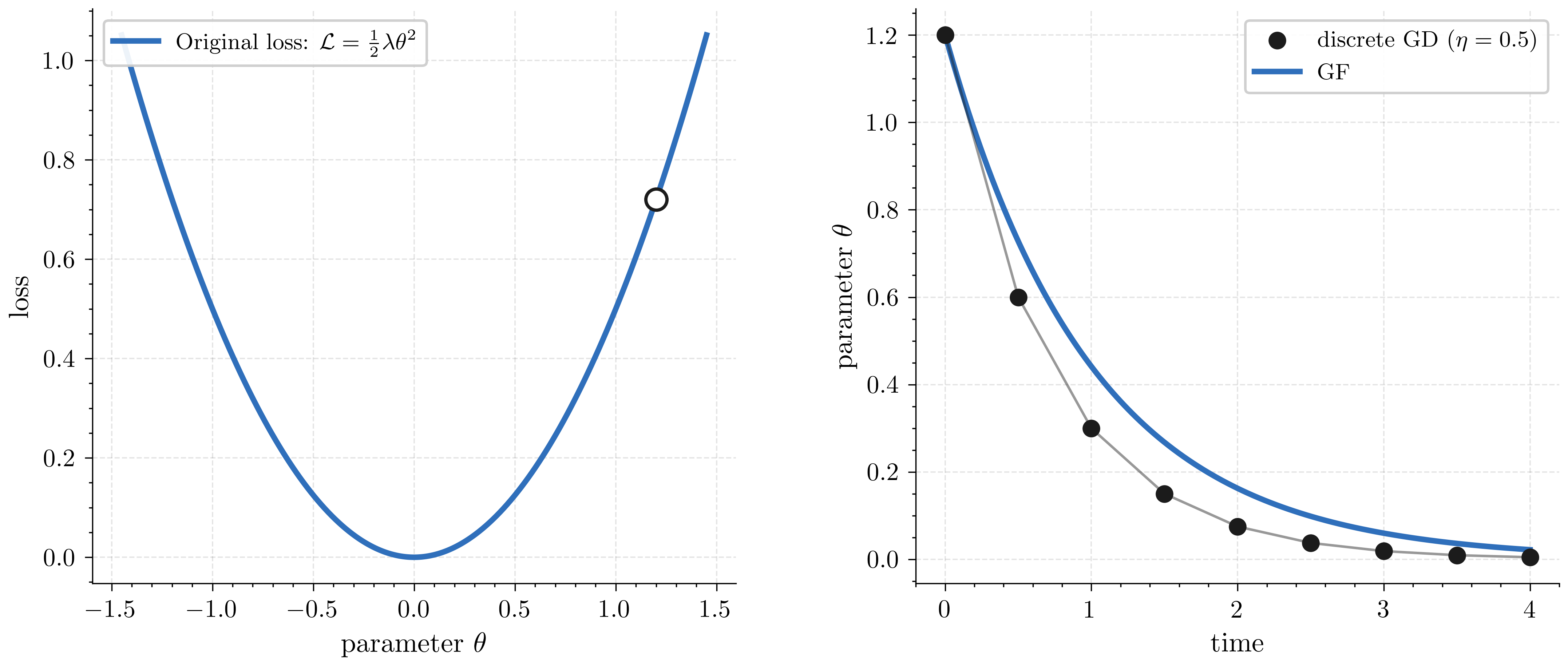
Left: the quadratic bowl L(θ)=2λθ2 and the starting point θ0=1.2. Right: parameter trajectories over time: GF (blue, continuous) and discrete GD (black dots, plotted at times t=kη with η=0.5). Note that the two paths do not match. In the case of our quadratic loss, GD approaches the minimum more quickly than GF – this is because GD locks in the starting gradient for the entire step, while GF’s gradient continuously shrinks as ∣θ∣ decreases.
The modified quadratic
From the above analysis, we see that gradient descent lands at θGD=(1−ηλ)θ0, while gradient flow lands at θflow=(1−λη+2λ2η2+O(η3))θ0. The mismatch primarily stems from the extra second-order term in gradient flow: 2λ2η2θ0. Note that this extra (positive) term causes gradient flow to move slightly less far down the quadratic bowl than gradient descent.
So, in order to construct a modified gradient flow that behaves similarly to gradient descent here, we can try making the bowl effectively steeper:
Lη(θ)=21(λ+2ηλ2)θ2.
We can now analyze how gradient flow behaves on this modified loss.
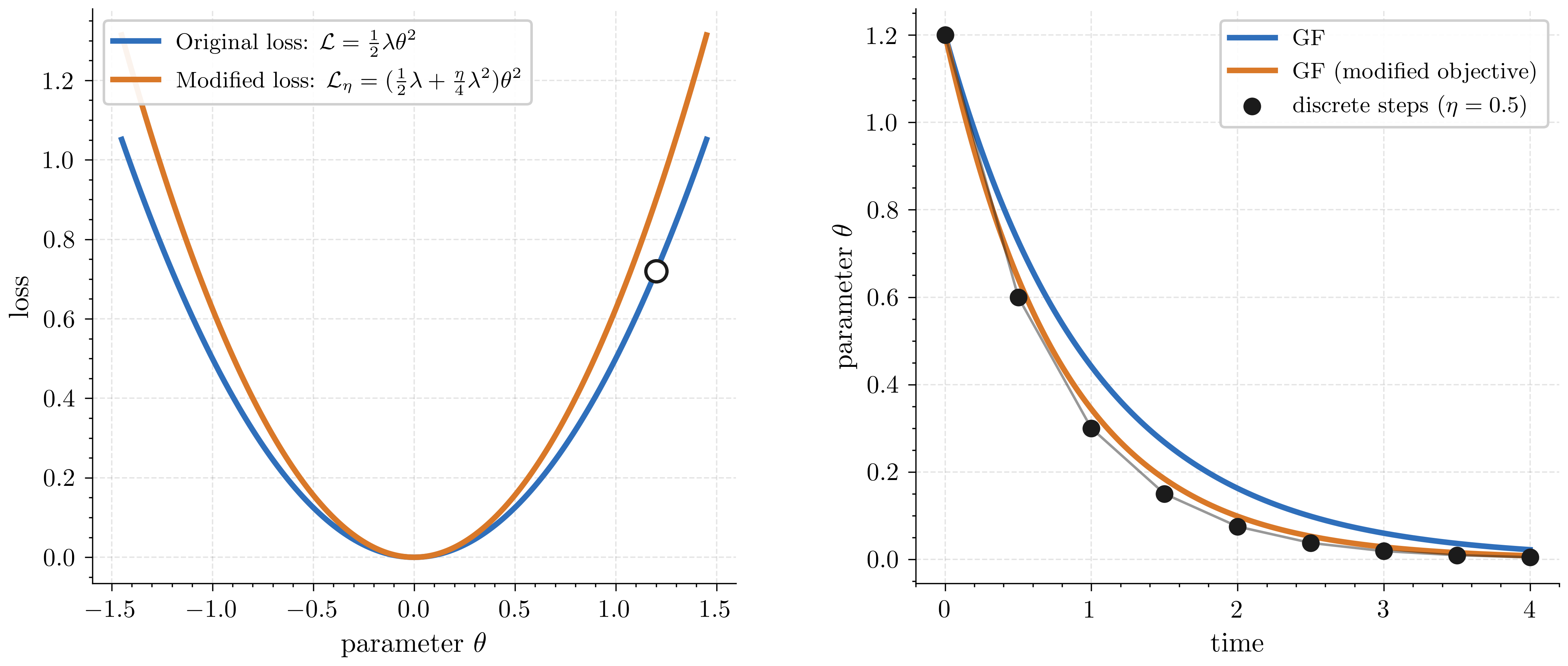
The order-η2 terms cancel, so gradient flow on the modified loss matches one gradient descent step on the original loss (up to order η2). Nice!
Rewriting the modified loss in terms of gradient norm
Let’s look back at the modified loss that we used. The modified loss is just the original loss plus one extra correction term:
Lη(θ)=original loss L(θ)21λθ2+finite-step correction4ηλ2θ2.
Since ∇L(θ)=λθ, we can write the extra term as
4ηλ2θ2=4η∥∇L(θ)∥2.
We will see that, in general, the modified loss can be written as
Lη(θ)=L(θ)+4η∥∇L(θ)∥2+O(η2).
Left: the original loss L(θ) (blue) and the modified loss Lη(θ) (orange), with λ=1 and η=0.5. Note that the modified loss is a slightly steeper bowl. Right: parameter trajectories over time: GF on the original loss (blue), GF on the modified loss (orange), and discrete GD (black dots). Note that GF on the modified loss now tracks the discrete GD steps more closely, compared to GF on the original loss.
The general case
Now we’ll try to generalize the modified loss construction.
We’ll denote the initial gradient as g:=∇L(θ0) and the initial Hessian as H:=∇2L(θ0).
We can write the endpoint of one gradient descent step as
θGD=θ0−ηg.
We can similarly write the endpoint of gradient flow on the original loss as
θflow=θ0−ηg+2η2Hg+O(η3).
Note that, just like in our toy quadratic case, gradient descent and gradient flow agree up to first order in η, but disagree at order η2 and higher. Gradient flow has an extra second-order term: 2η2Hg.
Now we try a nearby loss whose first correction is proportional to the step size:
Lη(θ)=L(θ)+ηR(θ)+O(η2),
where R is the correction term.
For gradient flow on this modified loss, initial velocity is
To match θGD=θ0−ηg through order η2, we need the η2 term to vanish; i.e., we need
∇R(θ0)=21Hg.
A function with this gradient is
R(θ)=41∥∇L(θ)∥2.Proof
Write R coordinate-wise as
R(θ)=41i∑(∂θi∂L(θ))2.
Differentiate with respect to coordinate θj:
∂θj∂R(θ)=21i∑∂θi∂L(θ)∂θj∂θi∂2L(θ).
At θ0, this becomes
∂θj∂R(θ0)=21i∑Hjigi.
That is the jth coordinate of 21Hg. Therefore ∇R(θ0)=21Hg.
Thus
Lη(θ)=L(θ)+4η∥∇L(θ)∥2+O(η2).
References
References are listed in alphabetical order.
Implicit gradient regularization[link] David Barrett and Benoit Dherin. International Conference on Learning Representations. 2021.
Neural mechanics: Symmetry and broken conservation laws in deep learning dynamics[link] Daniel Kunin, Javier Sagastuy-Brena, Surya Ganguli, Daniel LK Yamins, and Hidenori Tanaka. International Conference on Learning Representations. 2021.
On the origin of implicit regularization in stochastic gradient descent[link] Samuel L Smith, Benoit Dherin, David Barrett, and Soham De. International Conference on Learning Representations. 2021.
Neural thermodynamics: Entropic forces in deep and universal representation learning[link] Liu Ziyin, Yizhou Xu, and Isaac L. Chuang. Advances in Neural Information Processing Systems. 2025.