Zero-knowledge: theoretical foundations I

This summer, I’ve been studying the field of zero-knowledge. Zero-knowledge (ZK) is a subject that’s picked up a lot of hype lately, as its practical applications keep being discovered all over the web3 landscape. However, before diving into these recent applications of ZK, I wanted to first understand the theoretical foundations of ZK. The theory behind ZK is itself very beautiful, and worthy of study even independent of its applications in the real world.

The vast majority of this post (and subsequent ones) is my summarization of the amazing lectures from Bar Ilan’s 2019 Winter School. These lectures are presented by ZK gods, and are amazingly clear and well organized. I highly recommend watching them for anyone interested in understanding ZK theory, and full credit for the content of this post goes to the organizers of the course.

Thanks to my professor Tal Malkin for helping me understand this material, and thanks to my buddies Arnold and Raghav for proofreading this post.

What’s a proof?

Suppose Alice knows that some statement $s$ is true. Suppose that Bob does not yet know that $s$ is true. How can Alice “prove” to Bob that $s$ is true?

Well, in many cases, Alice can write down a logical explanation of how she knows that $s$ is true. Bob can then read this explanation, and also be convinced that $s$ is true.

For example, suppose $s$ to be the statement “$289$ is a square” (or in mathematical notation: “$\exists w \in \mathbb{N}$ such that $w^2 = 289$”). A simple proof that Alice could write down and send to Bob is the following:

• Let $w = 17$
• Then $w^2 = 17^2 = (10 + 7) * (10 + 7) = (10^2) + 2 (10 * 7 ) + (7^2) = 100 + 140 + 49 = 289$

There are two important aspects of the above proof to point out:

1. [non-interactive] The proof does not require interaction between Alice and Bob.
   • Alice can simply write her argument on a piece of paper, hand it to someone, and then walk away. The proof does not require Bob to ask questions or interact with Alice in any way. All he has to do is read Alice’s monologue to be convinced.
2. [non-zero-knowledge] Alice reveals to Bob not only that the statement is true, but also how the statement is true.
   • Alice shows Bob exactly which element $w$ satisfies the property $w^2 = 289$, namely $w =17$.
     • Such a $w$ is generally referred to as a “witness for $s$” – it’s a piece of information which makes the statement $s$ easy (efficient) to verify.

Ok, cool. Basically all proofs in mathematics are of this expository, non-interactive flavor. But this flavor of proof can’t be used to prove all statements – there are some statements for which it’s hard (or impossible) to explain exactly how they are true.

For example, suppose that Alice has a very sophisticated palate and can distinguish between the tastes of Coke and Pepsi. Bob cannot distinguish between them, and is not convinced that Alice can either. In this scenario, $s$ is the statement “Alice can distinguish between the tastes of Coke and Pepsi.” How can Alice prove this statement to Bob? She can’t simply explain to Bob how she distinguishes them, as language is insufficient to describe the sensation of taste precisely, especially when the two communicating parties have different palates!

While Alice can’t convince Bob of her sophisticated palate through direct explanation, she can convince him through the following game:

• Alice sets up two cups on a table.
• Alice pours Coke into the left cup, and Pepsi into the right cup. She then puts on a blindfold.
• Bob flips a coin:
  • If heads, Bob swaps the left and right cups.
  • If tails, Bob leaves the cups in their original configuration.
• Alice then tastes both cups, and says whether she thinks the cups were swapped or not.

If Alice can truly distinguish between Coke and Pepsi, the probability of her winning the game is $1$: she will always be able to tell whether the drink on the left is Coke or Pepsi, and therefore is always able to tell whether the cups were swapped or not.

On the other hand, if Alice cannot distinguish between Coke and Pepsi, then the probability of her winning the game is $1/2$: she cannot leverage taste to distinguish between the unswapped vs swapped scenario, and so her success probability is equivalent to correctly guessing the outcome of Bob’s coin flip.

If this game is played once and Alice wins, Bob may still not be convinced: even if Alice guessed randomly, she could have won with a 50% chance.

However, Alice and Bob can repeat the game $k$ times for some arbitrarily-large $k$ in order to amplify Bob’s confidence. In order for Alice to convince Bob of her discerning palate, she must win all $k$ rounds. If she loses even a single round, Bob will conclude that she has an ordinary tongue. With $k$ rounds of play, the probability of Alice deceiving Bob (in the case where Alice actually cannot distinguish between Coke and Pepsi) is equal to the probability of her randomly guessing Bob’s coin flip in all $k$ rounds: $2^{-k}$.¹

Let’s note two important aspects of the above proof:

1. [interactive] The proof requires interaction between Alice and Bob.
   • Bob introduces randomness to the protocol in the form of a coin flip. This coin flip determines the correct answer of the challenge (swap or not) that Alice must complete.
2. [zero-knowledge] Alice convinces Bob only that the statement is true, and does not reveal how the statement is true.
   • In this case, it’s not clear how the statement is true (there’s no obvious witness). But we will see examples where Alice does know some witness for the statement, and is yet still able to prove the statement without revealing the witness.

Summarizing proof types

From the two examples above, we’ve seen that there are two axes on which a proof can vary (the following statements are not precise and intended just to build up intuition – we’ll define the terms more formally in a bit):

1. Interactive vs non-interactive
   • In an interactive proof, Alice and Bob communicate with each other, and the protocol is usually non-deterministic (involves randomness).
   • In a non-interactive proof, Alice can complete her proof without any communication from Bob.
2. Zero-knowledge vs non-zero-knowledge
   • In a zero-knowledge proof, Alice convinces Bob that the statement is true, but does not reveal how the statement is true.
   • In a non-zero-knowledge proof, Alice convinces Bob that the statement is true by revealing how the statement is true.

We’ll see that there exist proofs which satisfy each of the $\{\text{interactive, non-interactive} \} \times \{\text{zk, non-zk} \}$ combinations. We’ll start by formally defining interactive proof systems, which will then enable us to define and understand zero-knowledge.

Interactive proof systems

An interactive proof system has two parties: a prover $P$, and a verifier $V$. The prover $P$ aims to convince the verifier $V$ of some statement “$x \in L$.” The proof should be quick and easy to verify, and we will therefore stipulate that the verifier $V$ runs in probabilistic-polynomial-time (PPT). On the other hand, we place no restrictions on running time of the prover $P$.

An interactive proof system for $L$ is a PPT algorithm $V$ and a function $P$ such that for all $x$:

• Completeness: if $x \in L$, then $\Pr[(P,V)$ accepts $x] \geq \frac{2}{3}$
• Soundness: if $x \notin L$, then for all $P^*, \Pr[(P^*,V)$ accepts $x] \leq \frac{1}{3}$

A few notes about this definition:

• The notation $P^*$ represents a “cheating prover” – a prover that does not necessarily behave the same as the $P$ specified by the proof system.
  • The soundness condition requires that, for all provers (even malicious ones), the probability of the verifier being convinced of a false statement is small.
• The completeness and soundness probabilities of $2/3$ and $1/3$ are just arbitrary constants that are used for convenience.
  • In general, the completeness and soundness probabilities can be bounded by any functions $c(\lvert x \rvert): \mathbb{N} \rightarrow [0,1]$ and $s(\lvert x \rvert): \mathbb{N} \rightarrow [0,1]$ such that:
    • $c(\lvert x \rvert) \geq \frac{1}{2} + 1/\mathrm{poly}(\lvert x \rvert)$ ​
    • $s(\lvert x \rvert) \leq \frac{1}{2} - 1/\mathrm{poly}(\lvert x \rvert)$ ​
  • Using such functions would yield an equivalent definition as the one above.
    • One definition can be transformed into another by amplification (next bullet point).
• By repeating the proof system $\mathrm{poly}(\lvert x \rvert)$ independent times, the completeness and soundness can be amplified to have negligible error: $c(\lvert x \rvert) - s(\lvert x \rvert) \geq 1 - 2^{- \mathrm{poly}(\lvert x \rvert)}$.

Example: IP for quadratic non-residuosity

We define the language of “quadratic residues in $\mathbb{Z}_N^*$”:

$$\mathsf{QR}_N = \{ x \in \mathbb{Z}_N^* \lvert \exists w \in \mathbb{Z}_N^* \text{ s.t. } x = w^2 (\text{mod } N)\}$$

Note that there’s an obvious way to prove that some quadratic residue $x$ is indeed a quadratic residue. One can simply reveal the witness $w$ which satisfies $x = w^2 (\text{mod } N)$.

Now we can define its complement,² the language of “quadratic non-residues in $\mathbb{Z}_N^*$”:

$$\overline{\mathsf{QR}_N} = \{ x \in \mathbb{Z}_N^* \lvert \nexists w \in \mathbb{Z}_N^* \text{ s.t. } x = w^2 (\text{mod } N)\}$$

How can one prove that some quadratic non-residue $x$ is indeed a quadratic non-residue? It’s not as obvious or simple as in the case of quadratic residues.

Turns out there’s a very simple and elegant interactive proof system for quadratic non-residuosity:

Interactive proof system for quadratic non-residuosity

[Source: Lecture 1, Slide 19[1]Introduction to zero knowledge [link]
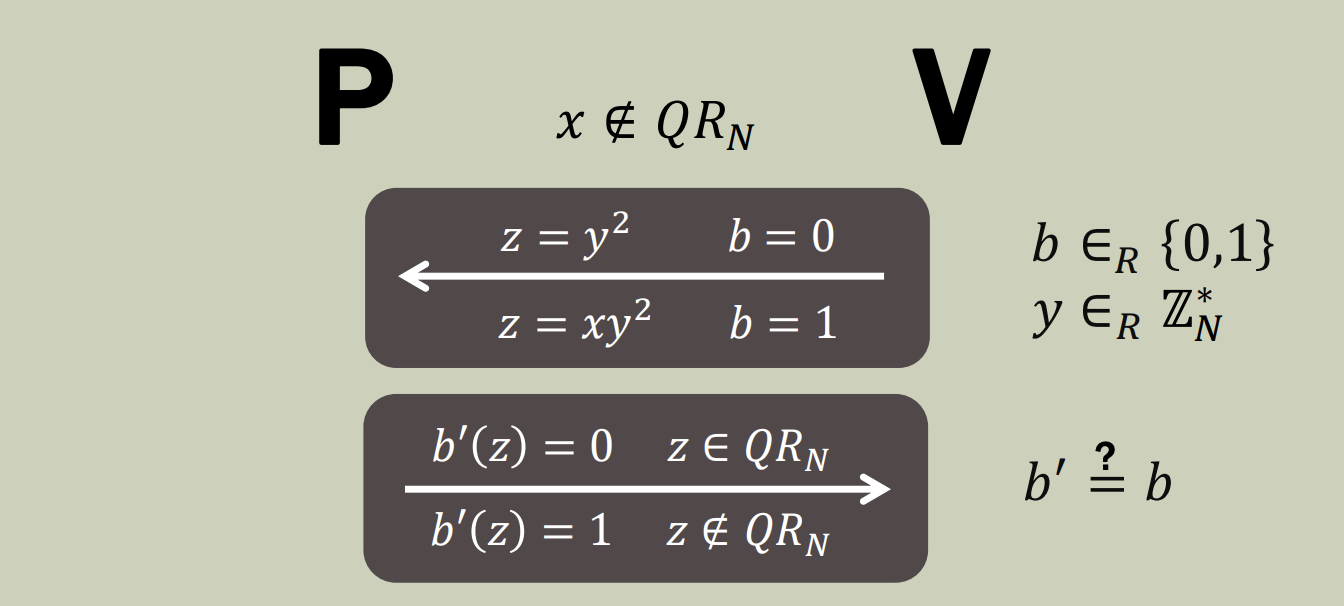
Alon Rosen. YouTube. 2019.]

• The verifier $V$ first randomly draws a bit $b \in \{ 0,1\}$, and an element $y \in \mathbb{Z}_N^*$.
  • If $b = 0$, then $V$ sends $z = y^2$ to $P$
  • If $b = 1$, then $V$ sends $z = x y^2$ to $P$
• The prover $P$ receives $z$ and checks if $z \in \mathsf{QR}_N$
  • If $z \in \mathsf{QR}_N$, $P$ sends $b'=0$ to $V$
  • If $z \notin \mathsf{QR}_N$, $P$ sends $b'=1$ to $V$
• The verifier $V$ checks if $b' = b$
  • If $b' = b$, then $V$ accepts
  • If $b' \neq b$, then $V$ rejects

Completeness:

• Suppose $x \notin \mathsf{QR}_N$
  • When $b=0$, $z = y^2 \in \mathsf{QR}_N \implies P$ sends $b'=0 \implies V$ accepts
  • When $b=1$, $z = xy^2 \notin \mathsf{QR}_N \implies P$ sends $b'=1 \implies V$ accepts
    • To see why $xy^2 \notin \mathsf{QR}_N$:
      $xy^2 \in \mathsf{QR}_N \implies \exists r \text{ s.t. } xy^2 = r^2 (\text{mod } N) \implies x = (r/y)^2 (\text{mod } N) \implies x \in \mathsf{QR}_N$
  • Therefore, $\Pr[(P,V) \text{ accepts } x] = 1$

Soundness:

• Suppose $x \in \mathsf{QR}_N$
  • Both $z = y^2 \in \mathsf{QR}_N$ and $z = xy^2 \in \mathsf{QR}_N$
  • $z$ in both cases is effectively uniformly randomly drawn from $\mathsf{QR}_N$, and reveals no information about $b$
  • Therefore, the best a malicious prover can do is try to guess $b'=b$ randomly:
    • $\forall P^*, \Pr[(P^*,V) \text{ accepts } x] = \Pr_b[P^*(z)= b] = 1/2$​

In a single round, the soundness error is $1/2$. Note that this does not actually satisfy the definition of soundness that we gave above, as the definition requires soundness error to be at most $1/3$.

The soundness of the protocol can be improved using a process called amplification: we can repeat the protocol for $k$ rounds, each with independent randomness, and have $V$ accept only if all rounds succeed. In this extended protocol, the probability of a cheating prover fooling $V$ (i.e. guessing $V$’s random bit) in all $k$ rounds is $2^{-k}$. Since $V$ runs in polynomial time, we can afford to run the protocol with $k = \mathrm{poly}(\lvert x \rvert)$ rounds, and therefore achieve soundness error $2^{-\mathrm{poly}(\lvert x \rvert)}$.

This example demonstrates the potential power of interactive proofs: for some languages, a simple non-interactive proof may not exist, while a simple interactive proof does.

Zero-knowledge

Finally, the time is upon us to define one of the coolest ideas in all of theoretical computer science: zero-knowledge.

Suppose Alice is trying to prove some statement $s$ to Bob. As mentioned in the introduction, a zero-knowledge proof should reveal no additional information to Bob, other than the fact that $s$ is true. In particular, Bob should not learn how $s$ is true – only that it is true.

Now, how do we formally define what it means for Bob not have learned any “additional information” from his interaction with Alice? Well, we could say that Bob doesn’t learn any new “additional information” if he could have known that information himself, without his interaction with Alice.

But now, how do we formally define what it means for Bob to have “known it himself” without the interaction? Well, we can say that Bob could output (“write down”) the information himself.

So, this means that, if the statement $s$ is true, Bob should be able to output, or “simulate”, his interaction with Alice, without actually interacting with Alice. For if Bob could not himself produce the information provided by Alice, then that information should be considered “additional knowledge” revealed by Alice.

This is the gist of the definition. In place of Bob, we use a randomized algorithm $S$ known as the “simulator”, which simulates the interaction between the prover and verifier, and outputs a transcript of this interaction.

Notation:

• $S(x) :=$ the distribution of transcripts output by the simulator $S$ when run on input $x$
• $(P,V)(x) :=$ the distribution of transcripts (ordered sequences of messages sent between $P$ and $V$) when the protocol $(P,V)$ is run on input $x$
• $S(x) \cong (P,V)(x)$ means that the distribution $S(x)$ is the same as the distribution $(P,V)(x)$

An interactive proof system $P, V$ for $L$ is honest-verifier zero-knowledge if there exists a probabilistic simulator $S$, running in expected polynomial time,³ such that $\forall x \in L$, $S(x) \cong (P,V)(x)$.

Note that this definition has a bit of a caveat: it only considers an honest verifier, i.e. a verifier who obeys the behavior specified in the protocol. In the real world, this is not really useful, as some verifier could be malicious and try to extract extra information from the prover by deviating from the specified protocol. We want to have a stronger definition that protects against this rogue-verifier (denoted as $V^*$) as well:

An interactive proof system $P, V$ for $L$ is perfect zero-knowledge if for all PPT $V^*$, there exists a probabilistic simulator $S$, running in expected polynomial time, such that $\forall x \in L$, $S(x) \cong (P,V^*)(x)$.

This definition is honestly super weird and hard to wrap your head around when you first learn about it (it was for me, at least), but the more you play around with it, the clearer and more beautiful it becomes. So let’s see it in action through an example.

Example: ZK IP for quadratic residuosity

Recall the language of “quadratic residues in $\mathbb{Z}_N^*$”:

$$\mathsf{QR}_N = \{ x \in \mathbb{Z}_N^* \lvert \exists w \in \mathbb{Z}_N^* \text{ s.t. } x = w^2 (\text{mod } N)\}$$

The following interactive proof system satisfies the definition of perfect ZK (and therefore honest-verifier ZK, since perfect ZK is a stronger definition):

Zero-knowledge interactive proof system for quadratic residuosity

[Source: Lecture 1, Slide 31[1]Introduction to zero knowledge [link]
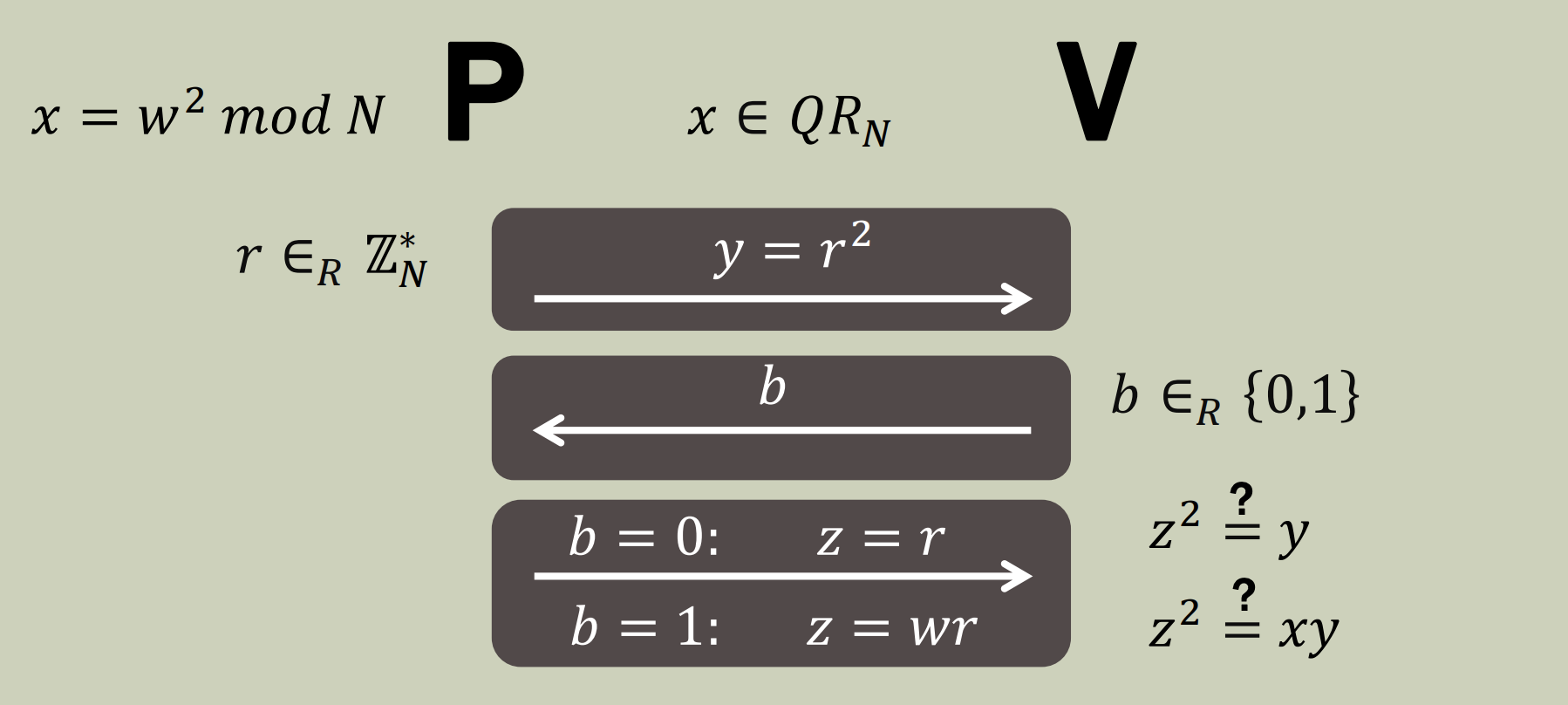
Alon Rosen. YouTube. 2019.]

• $P$ randomly draws an element $r \in \mathbb{Z}_N^*$, and sends $y = r^2$ to $V$
• $V$ randomly draws a bit $b \in \{ 0,1\}$, and sends it to $P$
• If $b = 0$:
  • $P$ sends $z = r$
  • $V$ accepts if $z^2 = y$
• If $b = 1$:
  • $P$ sends $z = wr$
  • $V$ accepts if $z^2 = xy$

Completeness:

• Suppose $x \in \mathsf{QR}_N$. Then $\exists w$ s.t. $x = w^2 (\text{mod } N)$
  • If $b = 0$, then $P$ sends $z = r$
    • Clearly $z^2 = r^2 = y$, and so $V$ accepts
  • If $b = 1$, then $P$ sends $z = wr$
    • Then $z^2 = (wr)^2 = w^2 r^2 = xy$, and so $V$ accepts

Soundness:

• Suppose $x \notin \mathsf{QR}_N$
  • Claim: $\nexists y \in \mathbb{Z}_N^*$ such that both $y \in \mathsf{QR}_N$ and $xy \in \mathsf{QR}_N$
    • To see this, suppose that both $y, xy \in \mathsf{QR}_N$. Then $\exists r, k \in \mathbb{Z}_N^*$ with $y = r^2 , xy = k^2$ (both equalities mod $N$). Then we could write $x = xy / y = k^2 / r^2 = (k/r)^2$, but this contradicts our assumption that $x \notin \mathsf{QR}_N$.
  • Thus, no matter what a dishonest prover $P^*$ does, at least one of $y$ or $xy$ must not be a quadratic residue.
    • If $y \notin \mathsf{QR}_N$, then $V$ will reject when $b=0$ (which happens w.p. 1/2)
    • If $xy \notin \mathsf{QR}_N$, then $V$ will reject when $b=1$ (which happens w.p. 1/2)
    • In other words, no matter what value of $y$ $V^*$ commits to, there is at least a probability of 1/2 that $V$ will reject
    • Therefore, we conclude that $\forall P^*, \Pr_b[(P^*,V) \text{ accepts } x] \leq 1/2$

Ok, we’ve proved that the protocol is an interactive proof system for $\mathsf{QR}_N$. Next, we need to prove that it is perfect zero-knowledge. To do this, we need to define a simulator $S$ that runs in expected polynomial time, and for all $x \in \mathsf{QR}_N$, the output of the simulator running on $x$ is the “same” as the protocol $(P, V)$ running on $x$. The key idea is that the simulator can “reverse” the order of the protocol: it can sample the challenge bit $b$ first, and can then craft $y$ to satisfy the challenge corresponding to $b$.

Consider the following simulator $S$:

1. Sample $z \leftarrow \mathbb{Z}_N^*$
2. Sample $b \leftarrow \{ 0, 1\}$
3. Set $y = z^2 / x^b$
4. Output $(y, b, z)$

The simulator’s output is randomly distributed over $(y, b, z)$ such that $y = z^2 / x^b$. The protocol’s output is randomly distributed over $(y, b, z)$ such that $z^2 = x^b y$. These distributions are the same, and so we’re done!

Hang on – not so fast. We forgot to consider what happens when there’s a rogue verifier $V^*$ that doesn’t follow the protocol! The above simulator is a proof for honest-verifier zero-knowledge, but we can also prove that the interactive proof system is perfect zero-knowledge.

Fix a malicious verifier $V^*$. The only part of the protocol that $V^*$ controls is the distribution of $b\text{:}$ instead of drawing $b$ at random, $V^*$ may set $b$ according to some function $b = V^*(y)$. We can adjust our simulator definition so that its distribution over $b$ matches that of the rogue verifier $V^*$.

Consider the following adjusted simulator $S'$:

1. Sample $z \leftarrow \mathbb{Z}_N^*$
2. Sample $b \leftarrow \{ 0, 1\}$
3. Set $y = z^2 / x^b$
4. If $b = V^*(y)$, then output $(y, b, z)$
5. Otherwise, repeat

Now our simulator’s output is randomly distributed over $(y, b, z)$ such that $y = z^2 / x^b$ and $b = V^*(y)$, which is the same distribution as the protocol running on $x$: $(P, V^*)(x)$. So now we’re done! Right?

No, not yet. We still need to argue that $S'$ runs in expected polynomial time. This is not immediately clear, since if $b \neq V^*(y)$ repeatedly, the code we wrote might run forever. We can argue that this is extremely unlikely though, and that the simulator actually only repeats a constant number of times in expectation.

The main idea is that the simulated distribution of $y$ is independent of $b$: $y$ is always a random, uniformly distributed element from $\mathsf{QR}_N$. When $b=0$, this is obvious, since $z^2$ represents a random element in $\mathsf{QR}_N$. When $b=1$, $z^2 x^{-1}$ is also a random element in $\mathsf{QR}_N$, since multiplying a group element by a random group element yields a random group element. Since $y$ is independent of $b$, $V^*(y)$ must also be independent of $b$, and so we have that on each iteration, $\Pr[b = V^*(y)] = 1/2$. Thus, the expected number of iterations for $S'$ is 2, and therefore the expected running time of $S'$ is 2 times the expected running time of $V^*$. Since $V^*$ runs in polynomial time, $S'$ satisfies the definitional requirement of running in expected polynomial time. Done!

We have shown that the above protocol is an interactive proof for $\mathsf{QR}_N$ with soundness error $1/2$, and that it satisfies perfect zero-knowledge. However, in the real world, we want to get soundness error down to a small value, like $2^{-\mathrm{poly}(\lvert x \rvert)}$. Recall that we can use sequential repetition to amplify the soundness error: we can repeat the protocol for $k = \mathrm{poly}(\lvert x \rvert)$ rounds. However, we need to be careful, and argue that this protocol with multiple repetitions preserves zero-knowledge. It is sufficient to build a simulator for the $k$-round protocol.

Consider the following simulator $S_k$:

• For round $i \in \{1, 2, ..., k\}$:
  1. Sample $z_i \leftarrow \mathbb{Z}_N^*$
  2. Sample $b_i \leftarrow \{ 0, 1\}$
  3. Set $y_i = z_i^2 / x_i^{b_i}$
  4. If $b_i = V^*(y_i, t_{i-1})$, then save $(y_i, b_i, z_i)$ and move on to the next round
     • Where $t_{i-1}$ represents all the previous message transcripts before round $i$
  5. Otherwise, repeat the current round $i$
• Output $(y_1, b_1, z_1, y_2, b_2, z_2, ..., y_k, b_k, z_k)$

Similar analysis⁴ yields that the expected running time of $S_k$ is 2 times the expected running time of $V^*$, and that $S_k$ therefore runs in expected polynomial time.

Cool! We’ve shown that the language $\mathsf{QR}_N$ has a perfect zero-knowledge interactive proof system, with soundness error $2^{-\mathrm{poly} (\lvert x \rvert)}$.

References

References cited in the text are listed first, in order of citation; additional references follow, ordered alphabetically.

1. Introduction to zero knowledge [link]
   Alon Rosen. YouTube. 2019.
2. The knowledge complexity of interactive proof systems [link]
   Shafi Goldwasser, Silvio Micali, and Charles Rackoff. SIAM Journal on Computing. 1989.
3. Lecture 15 - zero knowledge proofs [link]
   Boaz Barak. 2007.

Footnotes

1. Plugging in some concrete numbers: if there are $k=20$ rounds, then this probability is reduced to less than one-in-a-million: $2^{-20} = \frac{1}{1048576}$. Bob can of course specify the successful-cheating probability $p$ to be arbitrarily small, and then repeat the game $k = -\log{p}$ rounds to achieve such confidence. ↩

2. This is slightly imprecise. The complement of $\mathsf{QR}_N$ contains not only $\{ x \in \mathbb{Z}_N^* \lvert \nexists w \in \mathbb{Z}_N^* \text{ s.t. } x = w^2 (\text{mod } N)\}$, but also $\{ x \notin \mathbb{Z}_N^*\}$. Let’s just assume we’re only considering input $x$ values from $\mathbb{Z}_N^*$. ↩

3. We allow $S$ to run in expected polynomial time, rather than strict polynomial time. This is how the original GMR paper[2]The knowledge complexity of interactive proof systems [link]
   Shafi Goldwasser, Silvio Micali, and Charles Rackoff. SIAM Journal on Computing. 1989. defines it (see the last paragraph on page 10). We will revisit this part of the definition at a later stage, and see whether it’s possible to require the simulator to run in strict polynomial time. ↩

4. One needs to argue that $b_i$ is independent of $y_i$ and $t_{i-1}$. We already showed how to argue that $b_i$ is independent of $y_i$. $b_i$ is independent of $t_{i-1}$ since it is drawn fresh at each new round (i.e. knowing the transcripts of previous rounds cannot help $V^*$ predict $b_i$). ↩