Zero-knowledge: theoretical foundations II

This post is a continuation of a previous post, and will proceed with the material from Bar Ilan’s 2019 Winter School.

Introduction

In this post, our objective is to show that there exists a zero-knowledge interactive proof system for any language in NP. In order to do so, we will need to loosen our definition of zero-knowledge slightly. We will define statistical zero-knowledge and computational zero-knowledge, both of which are relaxations of perfect zero-knowledge (which we defined in the previous post). We will then take an NP-complete language, $\mathsf{HAM}$, and give an interactive proof system which satisfies computational zero-knowledge. It will then follow that any language in NP has a computational zero-knowledge proof, since any language in NP can reduced to an instance of $\mathsf{HAM}$.

The problem with perfect zero-knowledge for NP

Why do we need relaxations on our definition of perfect zero-knowledge at all? Why can’t we just construct proof system which satisfies perfect zero-knowledge for an NP-complete language?

Well it’s very very strongly believed that such a proof system cannot exist. In 1987, just a couple years after the original discovery of the concept of zero-knowledge, Fortnow [1]The complexity of perfect zero-knowledge [link]
Lance Fortnow. Proceedings of the Nineteenth Annual ACM Symposium on Theory of Computing. 1987. showed that if such a proof system exists, then the polynomial hierarchy collapses. Don’t worry if you don’t know what this means – just take my word that theoretical computer scientists believe very very strongly that the polynomial hierarchy does not collapse (quite similar to the strong belief that $\mathsf{P} \neq \mathsf{NP}$).

Thus, if we want to achieve zero-knowledge protocols for all languages in NP, we’re going to need to relax our definition of zero-knowledge.

In order to do tinker with the definition of zero-knowledge, we need to discuss some different notions of indistinguishability.

Notions of indistinguishability

Consider two random variables $X, Y$ over the domain $\Omega = \{ 0,1\}^{n}$. We want to formally define some notions of indistinguishability between these two variables.

The first notion is that of perfect indistinguishability: the distributions $X$ and $Y$ are exactly the same. Thus any algorithm will behave exactly the same whether its input is $X$ or $Y$.

$X,Y$ are perfectly-indistinguishable if for any algorithm $A$ (even a computationally unbounded algorithm), $\lvert \Pr[A(X)=1] - \Pr[A(Y)=1] \rvert = 0$.

Relaxing this definition a little, we get statistical indistinguishability: the distributions $X$ and $Y$ are almost the same, and their difference is bounded by a negligible value. Any algorithm will behave almost the same whether its input is $X$ or $Y$.

$X,Y$ are statistically-indistinguishable if for any algorithm $A$ (even a computationally unbounded algorithm), $\lvert \Pr[A(X)=1] - \Pr[A(Y)=1] \rvert \leq \epsilon(n)$, for some negligible function $\epsilon(n)$.

In the real world, it is reasonable to assume adversaries have limited computation power. We can apply this idea to get computational indistinguishability: any polynomially-bounded algorithm will behave almost the same whether its input is $X$ or $Y$.

$X,Y$ are computationally-indistinguishable if for any PPT algorithm $A$, $\lvert \Pr[A(X)=1] - \Pr[A(Y)=1] \rvert \leq \epsilon(n)$, for some negligible function $\epsilon(n)$.

Relaxing perfect zero-knowledge

Now that we have these relaxed notions of indistinguishability, we can use them to define a relaxed notion of zero-knowledge.

First recall the definition of perfect zero-knowledge:

An interactive proof system $P, V$ for $L$ is perfect zero-knowledge if for all PPT $V^*$, there exists a PPT simulator $S$ such that $\forall x \in L$, $S(x) \cong (P,V^*)(x)$.

Note that this definition requires the simulator’s output and the transcript to be perfectly-indistinguishable.

We can relax this to only require them to be statistically-indistinguishable:

An interactive proof system $P, V$ for $L$ is statistical zero-knowledge if for all PPT $V^*$, there exists a PPT simulator $S$ such that $\forall x \in L$, $S(x) \cong_S (P,V^*)(x)$.

However, it turns out that this definition is still not loose enough to use for NP. Fortnow [1]The complexity of perfect zero-knowledge [link]
Lance Fortnow. Proceedings of the Nineteenth Annual ACM Symposium on Theory of Computing. 1987. additionally showed that if there exists statistical zero-knowledge proofs for all problems in NP, then the polynomial hierarchy collapses.

Thus, we need another level of relaxation. This time, we allow the simulator’s output and the transcript to be computationally-indistinguishable:

An interactive proof system $P, V$ for $L$ is computational zero-knowledge if for all PPT $V^*$, there exists a PPT simulator $S$ such that $\forall x \in L$, $S(x) \cong_C (P,V^*)(x)$.

This definition will be loose enough, as we will be able to show that every language in NP has a computational zero-knowledge proof system. We’re almost ready to show such a construction, but we need to first discuss an important tool: commitment schemes.

Commitment schemes

A commitment scheme is a two-phase protocol between two parties: a committer, and a receiver. The idea is to have the committer commit to some value $m$ without revealing to receiver what $m$ is. To achieve this, the committer computes some value $c = \mathsf{Com}(m,r)$ (where $r$ is some randomness) and sends $c$ to the receiver. At a later time, the committer can “decommit”, revealing the original message $m$ and randomness $r\text{:}$ $\mathsf{Dec}(c) = (m, r)$. The receiver can verify that $c = \mathsf{Com}(\mathsf{Dec}(c))$.

There are a couple properties that are desirable for commitment schemes to have:

1. Hiding: the receiver should not be able to learn any information about the committed message $m$ from seeing the commit value $c$
2. Binding: the committer should be bound to the originally committed message $m$

For each of these properties, we can define them using a computationally unbounded model (“statistical”), or a computationally bounded model (“computational”).

A commitment scheme $\mathsf{Com}$ is statistically-hiding if for all pairs of distinct messages $m_1, m_2$, $\mathsf{Com}(m_1) \cong_S \mathsf{Com}(m_2)$.

A commitment scheme $\mathsf{Com}$ is computationally-hiding if for all pairs of distinct messages $m_1, m_2$, $\mathsf{Com}(m_1) \cong_C \mathsf{Com}(m_2)$.

To formally define binding, we’ll describe the “binding game.” Given two distinct messages $m_1, m_2$, an algorithm $C$ “wins the binding game” if $C$ generates values $c, r_1, r_2$ such that $\mathsf{Com}(m_1, r_1) = c = \mathsf{Com}(m_2, r_2)$.

A commitment scheme $\mathsf{Com}$ is statistically-binding if for any algorithm $C$ (even a computationally unbounded one), for all pairs of distinct messages $m_1, m_2$, $\Pr[C \text{ winning the binding game}] \leq \epsilon(n)$, where $\epsilon(n)$ is some negligible function.

A commitment scheme $\mathsf{Com}$ is computationally-binding if for any PPT $C$, for all pairs of distinct messages $m_1, m_2$, $\Pr[C \text{ winning the binding game}] \leq \epsilon(n)$, where $\epsilon(n)$ is some negligible function.

In an ideal world, it’d be great to have a commitment scheme which is both statistically-hiding and statistically-binding. However, such an awesome commitment scheme cannot exist. In fact, it’s a nice exercise to show that a scheme can never satisfy both properties simultaneously.

As a result, we are limited to working with two flavors of commitment schemes:

• statistically-hiding schemes, which are statistically-hiding and computationally-binding
• statistically-binding schemes, which are statistically-binding and computationally-hiding

Ok, we’re just about done with the dry definitions. Good job if you stuck through it. We’re almost at the finish line.

Hamiltonian cycles

Define $\mathsf{HAM} = \{ G | G \text{ contains a Hamiltonian cycle}\}$. A Hamiltonian cycle is a cycle through the graph which visits each vertex exactly once. This language $\mathsf{HAM}$ is NP complete – any language in NP can be reduced to $\mathsf{HAM}$ in polynomial time.

For this post, we will consider a graph with $n$ vertices as being represented by an $n \times n$ adjacency matrix, where the $(i,j)^{th}$ entry is a 1 if the graph contains the edge $i \rightarrow j$, and 0 otherwise.

Adjacency matrix representation of a graph G with a Hamiltonian cycle w (bolded)

[Source: Lecture 2, Slide 25[2]Zero knowledge for all NP [link]
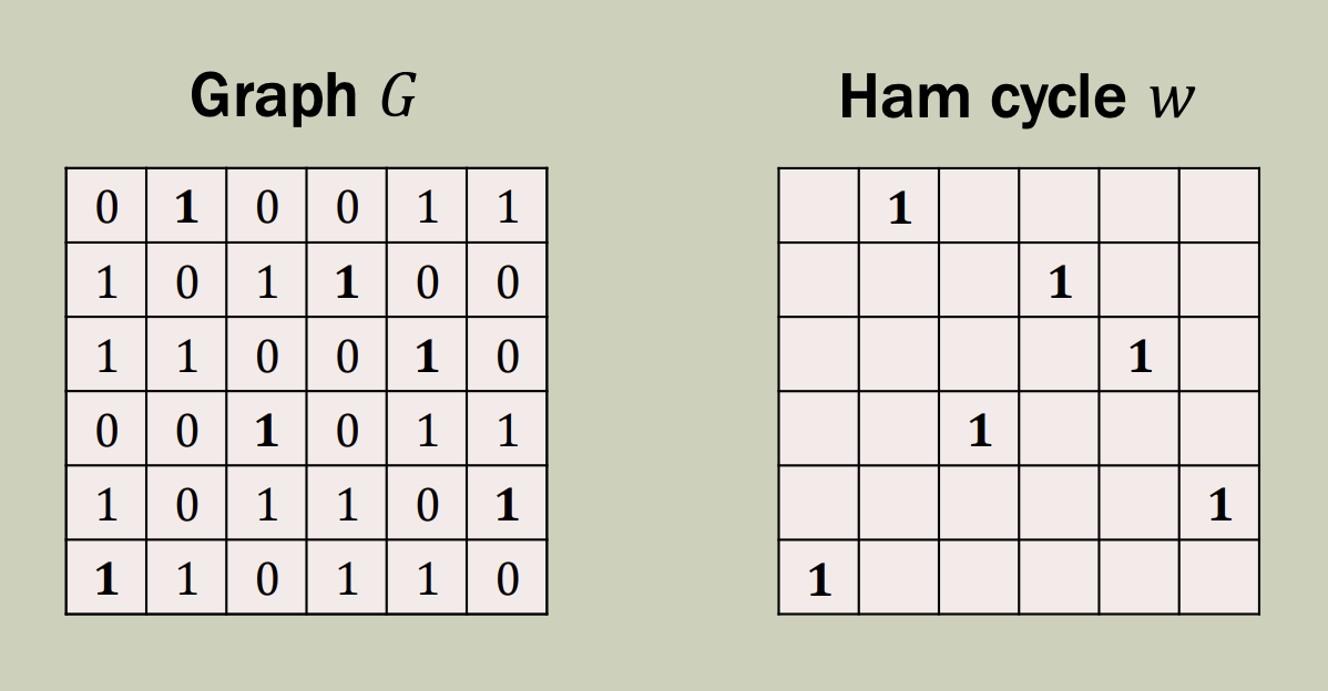
Alon Rosen. YouTube. 2019.]

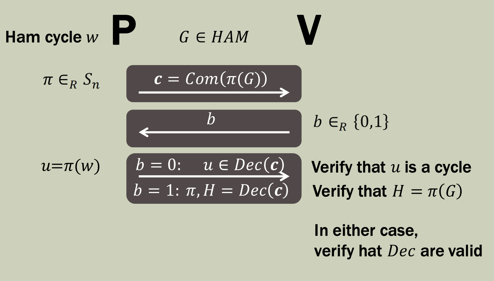
ZK proof for HAM

Computationally zero-knowledge proof for HAM

[Source: Lecture 2, Slide 27[2]Zero knowledge for all NP [link]
Alon Rosen. YouTube. 2019.]

• $P$ draws a random permutation $\Pi \in S_n$
• $P$ commits to $c = \mathsf{Com}(\Pi(G))$, and sends it to $V$
  • $\Pi(G)$ represents the original graph $G$ after permuting the vertices according to $\Pi$
  • $P$ can commit to $\Pi(G)$ by committing to each bit of the adjacency matrix for $\Pi(G)$
• $V$ then draws a random challenge bit $b \in \{ 0, 1\}$, and sends it to $P$
• If $b=0\text{:}$
  • $P$ only reveals the cycle within the permuted graph, i.e. that $u = \Pi(w) \in \mathsf{Dec}(c)$
    • $P$ does this by revealing only the particular bits in $\Pi(G)$ which correspond to the cycle $u = \Pi(w)$
  • $V$ verifies that $u \in \mathsf{Dec}(c)$ and that $u$ is a cycle
• If $b=1\text{:}$
  • $P$ sends the permutation $\Pi$ and reveals the permuted graph $H = \Pi(G)$
    • $P$ does this by revealing all the bits of $H=\Pi(G)$
  • $V$ verifies that $H = \mathsf{Dec}(c)$, and that $H = \Pi(G)$

Completeness: Completeness is straightforward. Suppose that $G$ has a Hamiltonian cycle $w$. A prover $P$ who follows the protocol honestly by drawing a random permutation $\Pi$ and sending $c = \mathsf{Com}(\Pi(G))$ will be able to answer both challenges correctly:

• $u = \Pi(w)$ is a cycle in $\Pi(G)$ since $w$ is a cycle in $G$. $u = \Pi(w)$ is contained in $H = \Pi(G)$, and therefore $u \in \mathsf{Dec}(c)$. So the $b=0$ challenge is successful.
• $H = \mathsf{Dec}(c)$ where $H=\Pi(G)$ by construction, so the $b=1$ challenge is successful.

Soundness: The claim is that if $\mathsf{Com}$ is statistically-binding, then soundness holds.

Assume that $G \notin \mathsf{HAM}$. Now suppose for contradiction that $\Pr_b[(P^*, V) \text{ accepts } G] > 1/2$. Then it must be the case that both challenges succeed, and hence $u$ is a Hamiltonian cycle in $H$ and $H = \Pi(G)$. But then $\Pi^{-1}(u)$ would give a valid Hamiltonian cycle in $G$, which would imply $G \in \mathsf{HAM}$. This is a contradiction, and hence we conclude that $\Pr_b[(P^*, V) \text{ accepts } G] \leq 1/2$.

Note that this argument only holds if we assume $\mathsf{Com}$ to be statistically-binding. If not, then $P^*$ could commit to some value $c$, and then reveal different values (both compatible with $c$) depending on which challenge bit was sent by $V$. Remember that in this model, the computation of $P^*$ is not bounded. That’s why a computationally-binding commitment is not good enough here.

Computational zero-knowledge: We’ll construct a simulator $S^{V^*}(G)$ as follows:

1. Set $G_0 = u$ for some random cycle $u$ over $n$ vertices
2. Set $G_1 = \Pi(G)$ for some random permutation $\Pi \in S_n$
3. Sample $b$ randomly from $\{ 0, 1 \}$
   • If $b=0$, set $c = \mathsf{Com}(G_0)$
   • If $b=1$, set $c = \mathsf{Com}(G_1)$
4. If $V^*(c) = b$
   • If $b=0$, output $(c, b, u)$
   • If $b=1$, output $(c, b, (\Pi, G_1))$
5. Otherwise, repeat

The output of this simulator $S^{V^*}(G)$ is computationally-indistinguishable from a real transcript $(P, V)(G)\text{:}$

• The two distributions of the commit message $c$ are computationally-indistinguishable because the commitment scheme $\mathsf{Com}$ is computationally-hiding.
  • Note that if $\mathsf{Com}$ were not computationally-hiding, then a PPT adversary might be able to distinguish between $\mathsf{Com}(G_0)$ and $\mathsf{Com}(G_1)$, and could therefore distinguish between the commit $c$’s simulated distribution vs its transcript distribution (the simulator commits to the cycle $G_0$ about half of the time, while the real protocol always commits to the fully permuted graph $G_1$).
• The two distributions of the challenge bit $b$ are identical, as $S$ matches the distribution of $V^{*}$.
• The distributions of $u$ and $(\Pi, G_1)$, as they are drawn in effectively the same way (uniformly random) in both the simulator and the real protocol.

Next, we argue that if $\mathsf{Com}$ is computationally-hiding, then $\Pr_{c, b}[V^*(\mathsf{Com}(G_b)) = b] \approx 1/2$ (where the approximation sign $\approx$ indicates that the difference between the two values is negligible). If this were not the case, then $V^*$’s output distribution would be non-negligibly different when running on input $\mathsf{Com}(G_0)$ and $\mathsf{Com}(G_1)$, and therefore $V^*$ could distinguish between the two inputs $\mathsf{Com}(G_0)$ and $\mathsf{Com}(G_1)$. But this violates the assumption that $\mathsf{Com}$ is computationally-hiding.

From $\Pr_{c, b}[V^*(\mathsf{Com}(G_b)) = b] \approx 1/2$, it follows that the expected number of repetitions the simulator makes is 2 (this analysis is similar to that done in the previous post for the quadratic residuosity proof).

Alright! That’s it, we’re done!

Conclusion

We started by establishing a limitation of our definition of perfect zero-knowledge, namely that there cannot exist (well, we really strongly believe that there cannot exist) perfect zero-knowledge proofs for all languages in NP. This motivated us to relax our definition to computational zero-knowledge: zero-knowledge that holds for polynomially-bounded machines. We then defined commitment schemes and their useful properties, all in preparation for our zero-knowledge proof of $\mathsf{HAM}$.

$\mathsf{HAM}$ is an NP-complete language, meaning any language in NP can be mapped to $\mathsf{HAM}$ in polynomial time. Thus, if we can create a computational zero-knowledge proof for $\mathsf{HAM}$, then this proof can be used to prove any language in NP! And that’s indeed what we did! Using statistically-hiding commitment schemes, we constructed an elegant interactive proof for $\mathsf{HAM}$ satisfying computational zero-knowledge.

References

References cited in the text are listed first, in order of citation; additional references follow, ordered alphabetically.

1. The complexity of perfect zero-knowledge [link]
   Lance Fortnow. Proceedings of the Nineteenth Annual ACM Symposium on Theory of Computing. 1987.
2. Zero knowledge for all NP [link]
   Alon Rosen. YouTube. 2019.
3. How to prove a theorem so no one else can claim it [link]
   Manuel Blum. Proceedings of the International Congress of Mathematicians. 1986.
4. Computational indistinguishability [link]
   Ryan O’Donnell. YouTube. 2020.